Difference in friction curve; penalty formulation (Abaqus) vs ideal coulomb friction curve 1

[drennon236]

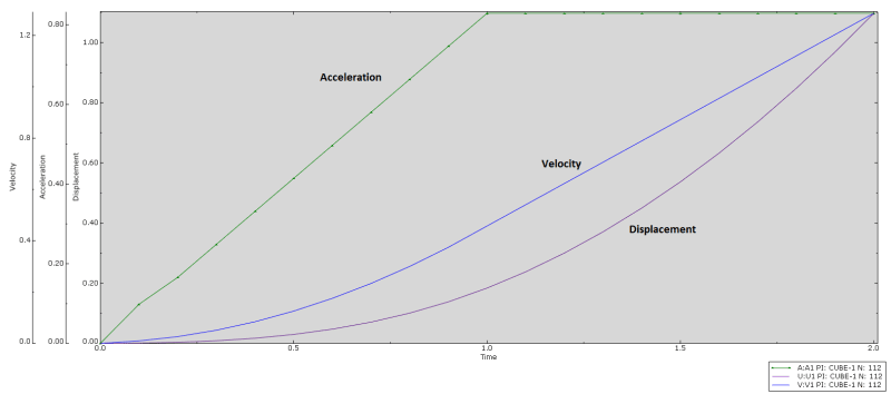
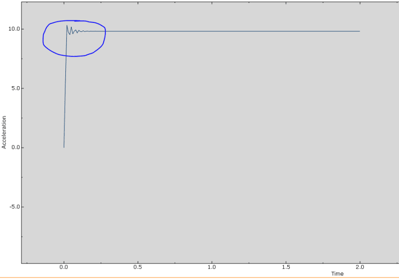
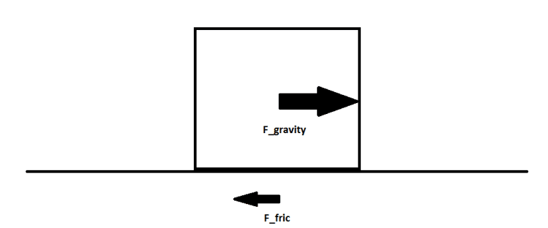
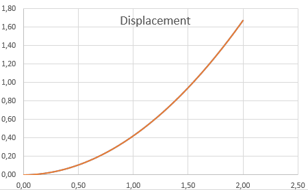
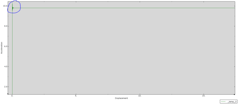
I am trying to understand the difference between the two models; The obvious one is that the penalty formulation has an elastic slip before reaching the slipping state, while the classic coulomb goes directly from sticking to slipping. I am working with a box on a plane, and I want to simulate a box on a plane which is pushed by a force, and then compare the Abaqus velocity, acceleration, and displacement vs time plot with analytical results. Will the results be similar? I tried running simulations, and got the same constant acceleration after elastic slip, but otherwise the Abaqus and analytical results do not match, and I am not sure if my model is incorrect or if the two models are incomparable.

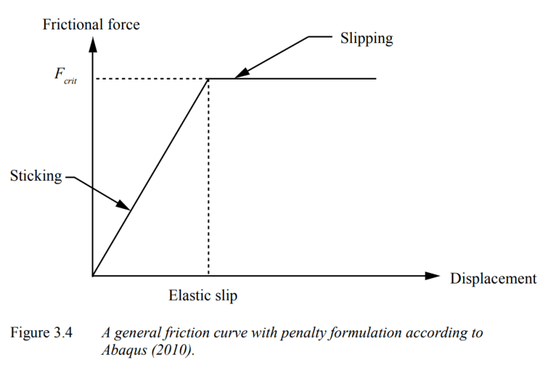
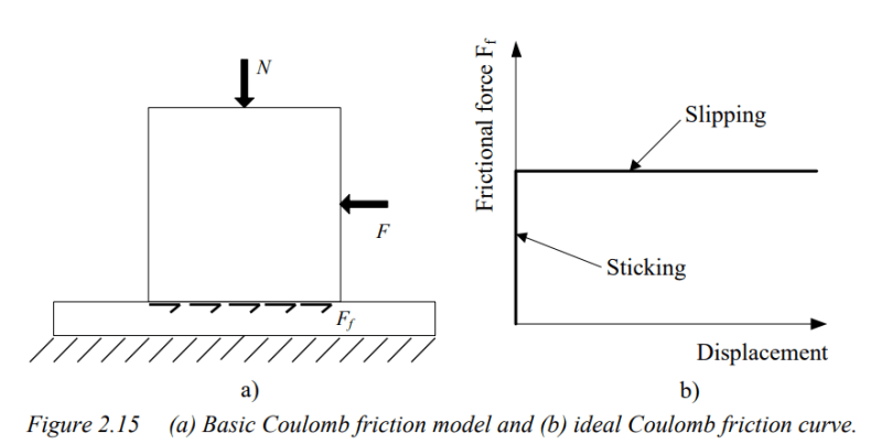
"In reality the elastic slip is assumed to correspond to the elastic displacement in the surface roughness." - is the elastic slip the displacement required for the box to "break free" from the plane? Does this elastic slip exist in the classic coulomb friction model?

 

[FEA way]

These two friction formulations (penalty and ideal Coulomb model) are analogous to elastic-perfectly plastic and rigid-perfectly plastic material models, respectively. Penalty formulation introduces finite elastic slip and thus the results are less accurate than those obtained with Lagrangian multipliers method. It's much better in terms of convergence, though.

 

[drennon236]

This is how my acceleration, velocity and displacement curve looks for the box on plane model with force pushing it horizontally. Since penalty method introduces finite elastic slip I assume this means I cannot get these results analytically? I will probably need experimental data to confirm the abaqus results then. Is elastic slip just some finite element model concept or is there a physical explanation for it?

 

[FEA way]

In case of models where friction is crucial for results, it is necessary to use Lagrange multipliers method to obtain accurate output. You can also try reducing maximum elastic slip setting for penalty method (to increase accuracy) but this may result in convergence difficulties.

 

[IceBreakerSours]

I have heard that argument of the choice between penalty and Lagrange multipliers before. Indeed, this is what the documentation or support representatives or even developers might tell you.

Firstly, I can understand it if a developer who only works on contact might make such an argument and it is a reasonable fact so long as you consider one axis (i.e., contact) out of many. However, there are other independent axes that play just as crucial a role in resolving contact - how smooth the contact pressure-overclosure relationship itself is, element behavior, and material stiffness. Therefore, I would argue that if one pays attention to multiple axes, then the choice isn't as binary as it might seem.

Secondly, Lagrange multipliers will resolve contact relatively accurately as opposed to penalty but you are adding additional degrees of freedom so the computational expense increases. If the model is small, you won't see a major impact on the wall clock time but if the model is large, then you will feel the pinch. Also, if you are choosing an implicit solution scheme, the stiffness matrix is ruined because of the off-diagonal terms. If the off-diagonal terms small in number or they are not significant in comparison with the diagonal terms, then your default solver may struggle but it may still get the job done. However, if the off-diagnoal terms are large in number or become significant, then the solver will crawl at which point you may have to switch to a non-default solution scheme. In other words, there are no free lunches.

Finally, based on my own personal experience, I have yet to come across a situation where penalty did not do a fine job.

*********************************************************
Are you new to this forum? If so, please read these FAQs:

http://www.eng-tips.com/faqs.cfm?fid=376

http://www.eng-tips.com/faqs.cfm?fid=1083

 

[drennon236]

Limiting the elastic slip with the penalty method I get this acceleration curve:

Could I ask what is the wavy part of the curve is before it converges - is it the springs trying to adjust to the allowed elastic slip?

And why doesn't the box simply fall off immediately?

 

[FEA way]

This marked part of the acceleration vs time plot looks like a typical numerical noise. Can you say more about this analysis ? What kind of step is that ? What are the boundary conditions, loads and contact settings ?

 

[drennon236]

This was a box on a plane model, but ultimately the goal is a grouted joint model.
Steel part inside and outside, and grout (concrete) in the middle.

-There is a normal pressure on the entire model to activate coulomb friction.
-Gravity is turned on, acting in the vertical direction.
-Inner steel part and concrete is encastered, will change this in the final model to only fix inner steel part.

-Surface to surface contact between the concrete and steel parts.
-Finite sliding (Any idea how the sliding formulation come into play here? I could not see a difference between finite and small sliding when I ran the model)

- Dynamic, Implicit with default load application so that I may limit the elastic slip. Will use quasi-static load application in the final model.

- Acceleration vs displacement curve of the outer steel part
- "Wavy" acceleration in the beginning again before it converges. Wondering if this is due to the penalty method and reduced elastic slip. The more I reduce the elastic slip the smaller the "wavy" part becomes.

 

[FEA way]

When it comes to sliding formulation, small sliding should be used only when you are absolutely sure that this assumption (of small sliding between the two surfaces) is valid. In such cases the numerical cost of the analysis will be lower. Otherwise, the results may be completely inaccurate.

I wouldn’t worry about this noise in acceleration curve. You can try eliminating it with filter applied to XY data, though.

 

[drennon236]

Just last question in this thread; when I go from small sliding to finite sliding I cannot use initial clearance to establish contact, which would give me a perfect initial contact condition, is there a way to get good contact conditions with finite sliding formulation? I tried doing the part sketches of the cylinder so theyre exactly touching, but this did not help much. Any ideas?

 

[FEA way]

You can use surface smoothing option, it's designed for such curved geometries. Also make sure that slave adjustment is enabled.