Frequency response in MatLab question

[T_M_S]

I’m doing my very first steps in MatLab (5 days since I had a first look at it).
I’d like to ask for a bit of help:
A bit of pretext: I’m trying to learn about vehicle ride dynamics using Adams car/ride 4 post shaker rig. I created a model representing amg gt4 car and excite the car with chirp input (constant velocity sine sweep).
I intend to postprocess the results in MatLab. My aim is to be able to get frequency response functions (FRF) – in a way described in attached pdf file (p.8, 7 post rig data analysis)

So far I’m able to import data to MatLab (exporting as table/spreadsheet from A/car) and create plots of power spectrum, psd and transfer function.
In that attached pdf author is using mathlab TFE function to get FRF. I’m using TFESTIMATE (but I tried TFE as well). Problem is that his results (Y axis) look very different to what I get – I get results in Db and his results are in… who knows. It looks like ratio to me.

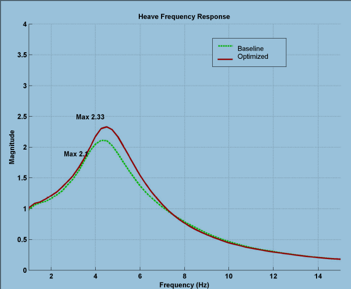
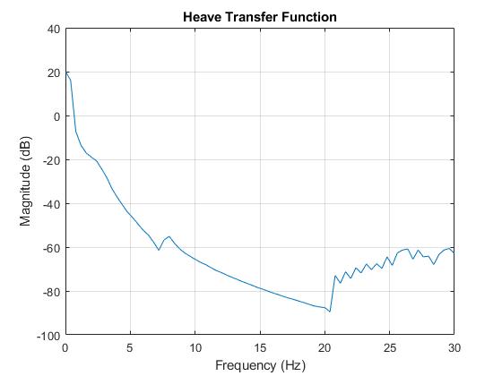
Is there a way that I can convert my Y axis from decibels to magnitude? There is a Matlab function db2mag but I can’t figure out how to apply it to my transfer function results.

Thank you,
Ted

 

[T_M_S]

Here's .mat file illustrating above question.

Thank you,
Ted

 

[T_M_S]

Here's live script file

Thank you,
Ted

 

[IRstuff]

decibels to magnitude

A decibel is a ratio; you need to find the reference level to convert to a magnitude

TTFN (ta ta for now)
I can do absolutely anything. I'm an expert!

https://www.youtube.com/watch?v=BKorP55Aqvg

faq731-376 forum1529 Entire Forum list

http://www.eng-tips.com/forumlist.cfm

 

[T_M_S]

Thank you, IRstuff.
Would you mind if I ask you to provide a little more detail regarding finding reference level?

Thank you,
Ted

 

[IRstuff]

That's a question for the shaker lab.

TTFN (ta ta for now)
I can do absolutely anything. I'm an expert!

https://www.youtube.com/watch?v=BKorP55Aqvg

faq731-376 forum1529 Entire Forum list

http://www.eng-tips.com/forumlist.cfm

 

[T_M_S]

Hmm...
Let me try again. I think that my poor English didn't allow me to express my question properly.
As far as I understand (please correct me if I'm wrong). Db is a ratio of magnitude of two signals expressed as 20*Log(A2/A1). Is there a way that I can get the results of tfestimate function to be expressed on linear scale?

Thank you,
Ted

 

[IRstuff]

Sure... Just undo the logarithm

TTFN (ta ta for now)
I can do absolutely anything. I'm an expert!

https://www.youtube.com/watch?v=BKorP55Aqvg

faq731-376 forum1529 Entire Forum list

http://www.eng-tips.com/forumlist.cfm

 

[T_M_S]

Thank you, IRstuff,
Problem is that this is my 7th day with MatLab and I know very little at this point. It seems to me that conversion to Db is sort of imbedded in tfestimate MatLab function and I can't figure out how to undo the logarithm in the result plot of this function. When I write the function it may look like this: tfestimate(y,x,[],[],[],Fs) in brackets I can input window size, overlap, etc. But I don't see Log10 in input arguments options and so I can't choose not to enter it... I suspect that I'm missing something very simple but I can't find it in help.
May I ask you to suggest how exactly I can write it in MatLab to get rid of Logarithm?

Thank you,
Ted

 

[GregLocock]

The dB reference value is 1, so if you were testing a spring mass system with a k of 100 it would start at 20 dB at 0 Hz.

It is a good idea to do the fft of each channel separately and then divide one by the other to check exactly what is going on scaling wise. Alternatively generate two known signals (say A and 10*A) and see what tfestimate gives.

Cheers

Greg Locock


New here? Try reading these, they might help FAQ731-376

http://eng-tips.com/market.cfm?

 

[GregLocock]

Having said that read the examples page for tfestimate, it does not automatically plot dB.

https://www.mathworks.com/help/signal/ref/tfestimate.html

Cheers

Greg Locock


New here? Try reading these, they might help FAQ731-376

http://eng-tips.com/market.cfm?

 

[IRstuff]

The dB reference value is 1

It's "1" of something, but the OP should already know that, since the transfer function required dividing the response by the input, so all the OP needs to answer is WHAT is the input?

TTFN (ta ta for now)
I can do absolutely anything. I'm an expert!

https://www.youtube.com/watch?v=BKorP55Aqvg

faq731-376 forum1529 Entire Forum list

http://www.eng-tips.com/forumlist.cfm

 

[T_M_S]

Thank you Greg,
There's definately a scaling mess which I have to fix first.
Regarding your 2nd reply - do you mean plotting abs of tfestimate? I didn't find any other way. May be it's my English playing tricks with me but I couldn't find any other way of plotting other than Db on y axis.

Thank you,
Ted

 

[GregLocock]

Yes, the default is to display dB, but if you take the output of tfestimate you can display that vector however you like, it's just a vector of complex numbers. ie

tfout=tfestimate(usual stuff in here);
plot(real(tfout),imag(tfout))

will give you a nyquist plot






Cheers

Greg Locock


New here? Try reading these, they might help FAQ731-376

http://eng-tips.com/market.cfm?

 

[T_M_S]

Thank you Greg,
That's what I'm doing now and with some fiddling with signal(exported from Adams) scaling things are starting to make sense.

Thank you,
Ted

 

[T_M_S]

In fact I was doing it differently:
tfout=tfestimate(usual stiff in here)
tfMag=abs(tfout)
tfPhase=angle(tfout)*57.3 to approximate phase in deg.
Then plot the above as two separate plots.
After rescaling Adams signals this gives me reasonable results with heave.
Doing it the way you suggested returns a very strange plot (sorry).
I will see how things work with other signals (pitch and cpl in particular) and report.

Thank you,
Ted

 

[cibachrome]

BTW: how is your porpoising problem study going ?

So: here's what I do for computing lateral handling analysis:
I have data channels from road & sim data with the usual names. They are segments of length power of 2. Beginning and ending with a zero input for a second or 2.
nfft = pow2(round(log2(length(STEER))));
sps = 100; % sample rate
nsegs = size(STEER,2);
for nseg=1 %:nsegs
[sstxy,f] = tfestimate(STEER,nseg), LATACC,nseg),rectwin(nfft),nfft/2,nfft,sps); % ayg by steer transfer function
[rolltxy,f] = tfestimate(LATACC,nseg),ROLL ,nseg),rectwin(nfft),nfft/2,nfft,sps); % roll by ay transfer function
[rollms2txy,f] = tfestimate(LATACC,nseg)*9.806,ROLL ,nseg),rectwin(nfft),nfft/2,nfft,sps); % roll by ay transfer function
[betatxy,f] = tfestimate(LATACC,nseg),SIDSLP,nseg),rectwin(nfft),nfft/2,nfft,sps); % beta by ay transfer function
[betasteertxy,f]= tfestimate(STEER ,nseg),SIDSLP,nseg),rectwin(nfft),nfft/2,nfft,sps); % beta by steer transfer function
[yawvtxy,f] = tfestimate(STEER,nseg), YAWVEL,nseg),rectwin(nfft),nfft/2,nfft,sps); % yawv by steer transfer function
[yawatxy,f] = tfestimate(STEER,nseg), YAWACC,nseg),rectwin(nfft),nfft/2,nfft,sps); % yaw accel by steer transfer function
[rollyawvtxy,f] = tfestimate(YAWVEL,nseg),ROLL ,nseg),rectwin(nfft),nfft/2,nfft,sps); % roll by yawvel transfer function
[rollswatxy,f] = tfestimate(STEER,nseg) ,ROLL ,nseg),rectwin(nfft),nfft/2,nfft,sps); % roll by steer transfer function

inx=find(f > 3.0 | f < .02);
f(inx)=[];
sstxy(inx)=[];
rolltxy(inx)=[];
rollms2txy(inx)=[];
betatxy(inx)=[];
betasteertxy(inx)=[];
yawvtxy(inx)=[];
yawatxy(inx)=[];
rollyawvtxy(inx)=[];
rollswatxy(inx)=[];

delta_f=f(2)-f(1);

handles.ss_gain = 100.*abs(sstxy); % convert to Bode form for gain
handles.ss_phase = angle(sstxy).*180/pi;
handles.yawv_gain = 100.*abs(yawvtxy);
handles.yawv_phase = angle(yawvtxy).*180/pi;
handles.yawa_gain = 100.*abs(yawatxy);
handles.yawa_phase = angle(yawatxy).*180/pi;
handles.roll_gain = abs(rolltxy);
handles.rollms2_gain = abs(rollms2txy);
handles.roll_phase = angle(rolltxy).*180/pi;
handles.rollms2_phase = angle(rollms2txy).*180/pi;
handles.beta_gain = abs(betatxy);
handles.beta_phase = angle(betatxy).*180/pi;
handles.betaswa_gain = 100*abs(betasteertxy);
handles.betaswa_phase = angle(betasteertxy).*180/pi;
handles.rollswa_gain = 100*abs(rollswatxy);
handles.rollswa_phase = angle(rollswatxy).*180/pi;
handles.rollyawv_gain = abs(rollyawvtxy);
handles.rollyawv_phase = angle(rollyawvtxy).*180/pi;
handles.f = f;
end

 

[T_M_S]

Thanks for great post Cibachrome,
I’m traveling right now but will reply as soon as I’m back home.

Thank you,
Ted

 

[cibachrome]

%Try this for the heave response with your data: Seems to work pretty well
load Question
[heavetxy,freq] = tfestimate(act_dz,heave,rectwin(nfft),nfft/2 ,nfft,Fs); % heave by act_dz transfer function
inx=find(freq > 20 | freq < .01);
freq(inx)=[];
heavetxy(inx)=[];
heave_gain = abs(heavetxy);
heave_phase = angle(heavetxy).*180/pi;

figure('name','T_M_S Porpoising Study','numbertitle','off','menubar','none')
subplot(2,2,1)
plot(freq,heave_gain,'o')
ylabel('Heave Gain (units ?)')
grid on
title('This is all you need to do Ted:')
subplot(2,2,3)
plot(freq,heave_phase,'o')
grid on
xlabel('Frequency (Hz.)')
ylabel('Phase (deg)')
sidetext('BillCobb zzvyb6@yahoo.com')

% Now go get the transfer function:
options = optimset('MaxFunEvals',1000000,'TolFun',.0000001,'Display','on');
FM0=[ .1 1 0.15 0.23 ]
for n=1: 5
[FM,error] = lsqcurvefit('splane2_fit',FM0 ,freq ,heave_gain,[],[],options);
heavesys =tf([FM(1:2 )],[FM(3:4) 1 ])
FM0=FM+ .001*rand(1);
end

N_1=num2str(FM(1));
N_0=num2str(FM(2));
D_2=num2str(FM(3));
D_1=num2str(FM(4));
D_0= '1';

f=.0 :.02:20;
[mag,phase]=bode(heavesys,f);
subplot(2,2,1)
hold on
plot(f,squeeze(mag),'b-')
mytexstr = ['$\frac{H(s)}{Z(s)}$ = $\frac{' N_1 's+' N_0 '}{' D_2 's^2+' D_1 's+' D_0 '}$']
text('string',mytexstr,'interpreter','latex','fontsize',15,'units','norm','pos',[.25 .75],'Fontweight','Bold');

[wn,z]=damp(heavesys);
subplot(2,2,3)
hold on
plot(f,squeeze(phase),'b-')
mytexstr = [ '$\omega_n = ' num2str(wn(1),3) ' Hz $']
text('string',mytexstr,'interpreter','latex','fontsize',12,'units','norm','pos',[.4 .7],'Fontweight','Bold');
mytexstr = [ '$\zeta = ' num2str(z(1),3) '$']
text('string',mytexstr,'interpreter','latex','fontsize',12,'units','norm','pos',[.4 .5],'Fontweight','Bold');

subplot(2,2,2)
bode(heavesys)
ylabel('Heave Response')
grid on

subplot(2,2,4)
step(heavesys,5)
ylabel('Heave Response (units ??)')
grid on

You'll need this: Note: I'm only using magnitude for fit criteria. phase floats
function [mag] = splane2_fit(FM,f)
sys = tf([FM(1:2 )],[FM(3:4) 1]);
mag = squeeze(bode(sys,f));

 

[cibachrome]

Anybody considered that the porpoising is a ride problem, not necessarily an aero problem ? Sure, aero can attenuate it, but the root cause seems to be something else.

BTW: Your 1000 Hz. sample rate is way overkill. What would help your activity is a longer data segment for a smaller delta_F frequency increment, multiple segments for ensemble averaging, adding a starting & ending signal of a second or 2, and a power of 2 number of samples. Some nonlinear effects smear the FFT data from the Question.mat file, but hopefully, you get the idea...

This is pitch by act_dz.