New Formula Help 1

[Kenja824]

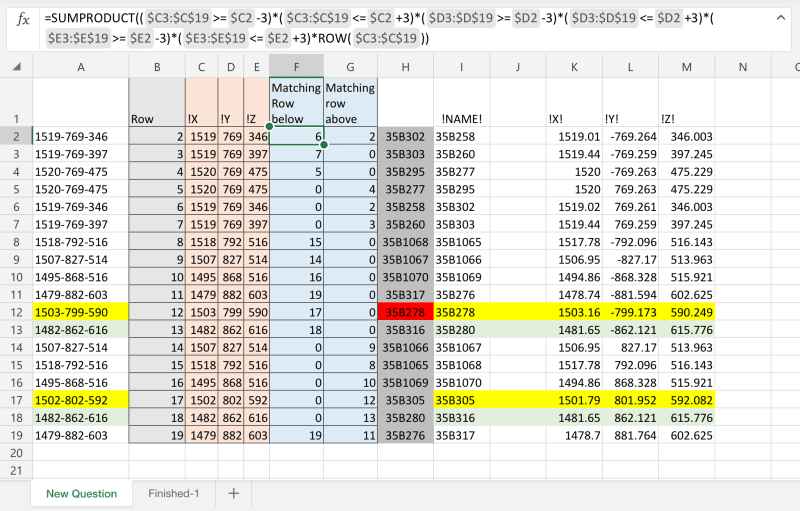
On the attached excel file (in the New Question tab) Is a list of spot numbers under the "!NAME!" header. To the right of those are three columns with the location of the weld spots in the XY and Z directions.

Column A has formulas that take the locations down to whole numbers and removes the negatives, then concatenates the results adding dashes between. This gives each spot a new ID number based on its location.

Column G has a formula that searches for another spot number that has the identical location ID and returns the name of that spot number.

The end result is that the G column will give us the opposite hand ID of the spot number in column H.

Basically the opposite hand spots will usually be in the same location, but if the original spot is in the positive direction for the Y direction, then the opposite will have a negative direction in the Y.


My Problem is that there is allowed up to a 3mm tolerance in all directions. My formulas only allow for less than .5mm tolerance because they round the numbers to whole numbers.


Is there a way using formulas that will find the opposite hand spot number if there is a 3mm difference in any or all of the directions?


You will notice tin the attached excel that I high lighted two spots in yellow, which should be opposite to each other. These are the example of spots being off but staying within their tolerance. My formulas will result in its own spot number because it cannot find a spot that is in the right location.

I have two spots in green. You will notice that these spots have each others numbers in the adjacent columns. This is what should happen if it is all correct.

If something like this takes VB coding that I can add to the file and add a new function to do the job, that would be just as good.


Thanks


Ken

http://www.OneGodLogic.com

My brain is like a sponge. A sopping wet sponge. When I use it, I seem to lose more than I soak in.

 

[SkipVought]

Ken,

Took your midweek bogdown question.

Uploaded your file with my additions:

3 separate columns for your spot values, just using the ROUND() function.
BTW, the Row column was just for looks, not necessary
Then a column to "match" values below with your tolerance
Then another to "match" values above

I didn't go any further.

This formula evaluates the X, Y & Z value in the row +/- 3 with the range of data BELOW and the other formula ABOVE. When there is a TRUE for X, Y & Z values in the range BELOW, then the ROW containing that "match" is calculated. The modification below says...
If the occurrence count is ONE then calculate the ROW else ZERO.

BTW, this method only works if there is ONE and only ONE Row solution. Otherwise, the formula will SUM the Row numbers. Therefore the formula must be modified to allow only ONE "match"...
[Pre]
=IF(
SUMPRODUCT(
($C3:$C$19>=$C2-3)*($C3:$C$19<=$C2+3)*
($D3:$D$19>=$D2-3)*($D3:$D$19<=$D2+3)*
($E3:$E$19>=$E2-3)*($E3:$E$19<=$E2+3)
)=1,
SUMPRODUCT(
($C3:$C$19>=$C2-3)*($C3:$C$19<=$C2+3)*
($D3:$D$19>=$D2-3)*($D3:$D$19<=$D2+3)*
($E3:$E$19>=$E2-3)*($E3:$E$19<=$E2+3)*
ROW($C3:$C$19)
),
0)
[/pre]

Skip,
[sub]
Just traded in my OLD subtlety...
for a NUance![/sub]

 

[BridgeSmith]

I got lost in most of that, but with the MROUND function, you can round to any increment you choose.

 

[SkipVought]

Ken,

I took it all the way, with the following assumptions:
The +/- 3 tolerance is to the actual !X!, !Y!, !Z! value.
There is a +!Y! for each -!Y!

So I'm using the values on the sheet without rounding.
In !Y! I'm comparing the product of the !Y! value and -1 to the comparison !Y! Range.

I use 2 sets of SUMPRODUCT():
[highlight #FCE94F]The set used for determining if I have ONE downward "match" OR ONE upward "match"[/highlight] returns a COUNT of rows that meet the tolerance comparison. The downward SUMPRODUCT() and the upward SUMPRODUCT() are summed.

If there is only ONE "match" downward OR upward, then I use [highlight #8AE234]the SUMPRODUCT() set that includes the Row()[/highlight] that is guaranteed to return only ONE Row number and not a sum of multiple rows. The downward SUMPRODUCT() and the upward SUMPRODUCT() are summed.

That unique row number is then used in the INDEX() function as the row number of the value in column I.

The formula in H2:
[pre]
=Index(I:I,
If(
[highlight #FCE94F]SUMPRODUCT(
(K3:K$19>=K2-3)*(K3:K$19<=K2+3)*
(L3:L$19>=(L2*-1)-3)*(L3:L$19<=(L2*-1)+3)*
(M3:M$19>=M2-3)*(M3:M$19<=M2+3))+
SUMPRODUCT(
(K1:K$2>=K2-3)*(K1:K$2<=K2+3)*
(L1:L$2>=(L2*-1)-3)*(L1:L$2<=(L2*-1)+3)*
(M1:M$2>=M2-3)*(M1:M$2<=M2+3))[/highlight]=1,
[highlight #8AE234]SUMPRODUCT(
(K3:K$19>=K2-3)*(K3:K$19<=K2+3)*
(L3:L$19>=(L2*-1)-3)*(L3:L$19<=(L2*-1)+3)*
(M3:M$19>=M2-3)*(M3:M$19<=M2+3)*
ROW(K3:K$19))+
SUMPRODUCT(
(K1:K$2>=K2-3)*(K1:K$2<=K2+3)*
(L1:L$2>=(L2*-1)-3)*(L1:L$2<=(L2*-1)+3)*
(M1:M$2>=M2-3)*(M1:M$2<=M2+3)*
ROW(K1:K$2))[/highlight],
0),
1)
[/pre]

This solution in your workbook on sheet New Question (2)

And there's one more thing I'd do to improve this solution. And that is to replace the 19 (the last row number) with an absolute reference to a cell that contains...

[tt]
=COUNTA(I:I)
[/tt]

...the row count of your !NAME! column.

Skip,
[sub]
Just traded in my OLD subtlety...
for a NUance![/sub]