han_cyuan
Structural
- Sep 20, 2023
- 31
You have entered a zero or negative density value. Abaqus allows non-physical data; however, most applications expect a positive density value and greater than 1.00000e-36 .
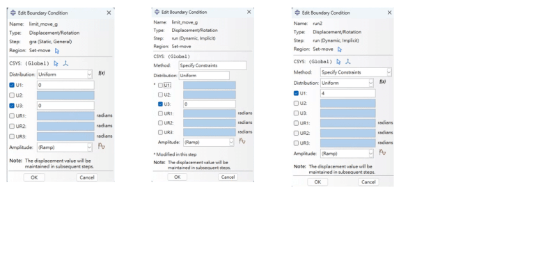
4 nodes associated with rigid bodies have boundary conditions prescribed at nodes other than the reference node. These boundary conditions will be transferred to the associated rigid body reference node.The reference nodes and the dependent nodes have been identified in node set WarnNodeOverconBoundRB.
Nodes belonging to 2 RIGID BODIES have boundary conditions prescribed at nodes other than the reference node. These boundary conditions indicate the rigid bodies cannot rotate about certain axes. Zero rotational boundary conditions have been added to these reference nodes.The reference nodes have been identified in node set WarnNodeOverconBoundRBRot.
Solver problem. Zero pivot when processing node ASSEMBLY.1 D.O.F. 4.
Solver problem. Zero pivot when processing node ASSEMBLY.1 D.O.F. 5.
Solver problem. Zero pivot when processing node 1 (assembly) D.O.F. 4
Solver problem. Zero pivot when processing node 1 (assembly) D.O.F. 5
Solver problem. Zero pivot when processing D.O.F. 4 of 1 nodes. The nodes have been identified in node set WarnNodeSolvProbZeroPiv_4_1_1_1_1.
Solver problem. Zero pivot when processing D.O.F. 5 of 1 nodes. The nodes have been identified in node set WarnNodeSolvProbZeroPiv_5_1_1_1_1.
The system matrix has 1 negative eigenvalues.
Solver problem. Zero pivot when processing node ASSEMBLY.1 D.O.F. 4.
Solver problem. Zero pivot when processing node ASSEMBLY.1 D.O.F. 5.
Solver problem. Zero pivot when processing node 1 (assembly) D.O.F. 4
Solver problem. Zero pivot when processing node 1 (assembly) D.O.F. 5
Solver problem. Zero pivot when processing D.O.F. 4 of 1 nodes. The nodes have been identified in node set WarnNodeSolvProbZeroPiv_4_1_1_2_1.
Solver problem. Zero pivot when processing D.O.F. 5 of 1 nodes. The nodes have been identified in node set WarnNodeSolvProbZeroPiv_5_1_1_2_1.
Solver problem. Zero pivot when processing node ASSEMBLY.1 D.O.F. 4.
Solver problem. Zero pivot when processing node ASSEMBLY.1 D.O.F. 5.
Solver problem. Zero pivot when processing node 1 (assembly) D.O.F. 4
Solver problem. Zero pivot when processing node 1 (assembly) D.O.F. 5
Solver problem. Zero pivot when processing D.O.F. 4 of 1 nodes. The nodes have been identified in node set WarnNodeSolvProbZeroPiv_4_1_1_3_1.
Solver problem. Zero pivot when processing D.O.F. 5 of 1 nodes. The nodes have been identified in node set WarnNodeSolvProbZeroPiv_5_1_1_3_1.
Solver problem. Zero pivot when processing node ASSEMBLY.1 D.O.F. 4.

