Continue to Site

Eng-Tips is the largest engineering community on the Internet

Intelligent Work Forums for Engineering Professionals

  • Congratulations KootK on being selected by the Eng-Tips community for having the most helpful posts in the forums last week. Way to Go!

Can a thicker model have a lower critical buckling load? 1

Status
Not open for further replies.

tugni925

Mechanical
Sep 14, 2020
107
I perform a linear buckling analysis for two similar geometries, where one model has thickness t = 0.01 m, and the other has thickness t = 0.035 m. Otherwise everything is exactly the same. The thinner model (t = 0.01m) however gives me a higher critical buckling load compared to thicker model (t = 0.035m)- could this be right? The slope in the linear region or Young's Modulus for both models seem to correspond well with previous studies, it is just that I'm getting lower buckling load as I increase the thickness.
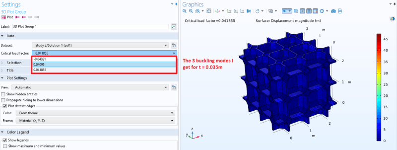
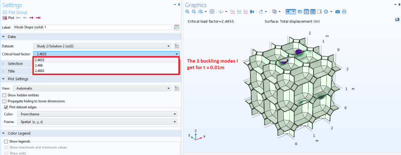
1_hiotbk.png


2_e1xzlo.png


Edit: I had to increase the Dimensions of the Krylov space from 0 to 300 to capture any buckling modes for the t = 0.035 m model.
 
Replies continue below

Recommended for you

what does "critical load factor" mean ? (immediately above your red rectangle)

when you change the thickness did you also change ...
1) the overall size, or
2) the size of the webs ?

another day in paradise, or is paradise one day closer ?
 
In Comsol critical load factor is the number by which you have to multiply your loads to reach buckling.

Try doing some buckling studies on a similar but simpler structure. This way you might be able to learn what to expect from these analyses.
 
this that saying that the 0.01m thick model is much stronger than the 0.035m model ?

it's hard (for me) to read the numbers but it looks like 2.4 for 0.01 and 0.04 for 0.035 model.

the -ve mode means imaginary mode ?

is it "odd" that the three modes (for each model) are close to this critical load factor ?

another day in paradise, or is paradise one day closer ?
 
You're right rb1957, 2.4 for 0.01 and 0.04 for 0.035 model. It should be the opposite, I suspect something is wrong with the solver as COMSOL support themselves did not seem to know either. I cant comment on -ve mode, but this model is made up of 3x3x3 identical parts put together. I will try to put them together as a beam and maybe the solver will have an easier time finding the buckling modes.
 
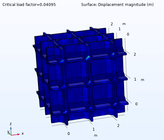
What do the buckling mode shapes look like for the 0.035 model? I can't see the deformed shape in your screen grab.

What loading have you applied - edge load, edge pressure, enforced displacement, or what? If you have used enforced displacement, the loads generated will be much higher for the thicker model, for the same displacement.

 
I have used a displacement of -0.01m in the x-direction. Mode shape looks like this:

1_pem8gj.png
 
Sigh. If you are applying the same enforced displacement to both models, the applied load on the thicker part will be much higher, hence the lower predicted eigenvalue.
 
That’s why I recommend starting from a simpler model. Maybe even regular pipe under compression. It will be much easier to understand its behavior in buckling analyses.
 
I get what you are saying, but here is why I am confused:

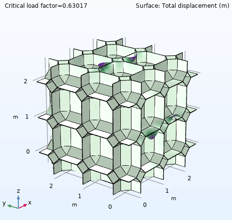
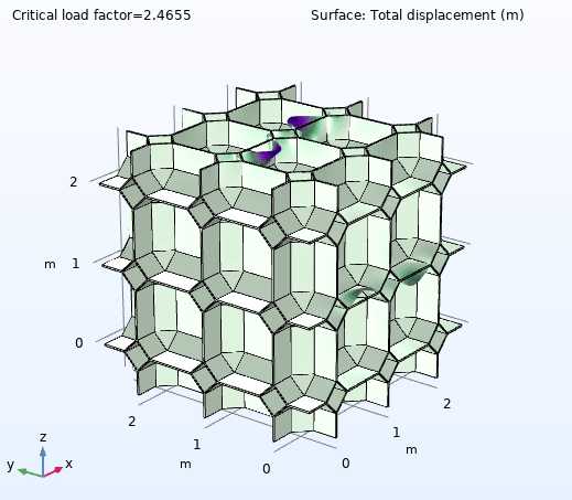
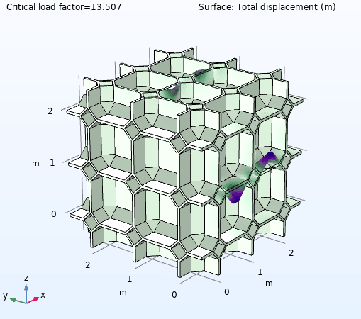
Here are three seperate models with thickness of t = 0.005m, 0.01m and 0.025m respectively, all have a displacement of -0.01m in the x-direction. As you can see the critical buckling load increases alongside the thickness.

t= 0.005 m
1_nukaim.png

t= 0.010 m
2_nashnh.png

t= 0.025 m
3_sxwrai.png


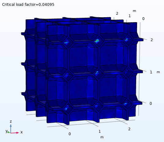
But then suddenly at thickness t=0.035m the buckling mode drops all the way to 0.04095?

4_i4w2iy.png
 
I plotted the stress strain curve of each buckling mode, and compared it with nonlinear buckling analysis data: Link. As you can see the slope or Youngs Modulus seem to match well for all three plots, but the linear model for t=0.035 seems to buckle at a much earlier point than the other two. What do you guys think?
 
I think there is a degeneration to the geometry. Make the thickness 0.1mm to check what it looks like.

Also, create a section through the part to show a representative sample of the hidden nodes where the problem exists, maybe with some more pixels to actually see what is happening.

 
so 0.005, 0.01, 0.025 trend as expected, and show the same mode.
but 0.035 bucks this trend and has a different mode shape ...

Am I right is seeing that the overall model size is constant as thickness changes ?
so the walls change size as the thickness increases ?

how is the model constrained ?

another day in paradise, or is paradise one day closer ?
 
So seems there was neither a problem with COMSOL or my model, but the cluster I ran the job on. I ran it on my computer and it gave me results as you would expect. I have no idea why it gives me wrong results running on the cluster though.
 
man! that is Weird !! Machine dependent error ??

another day in paradise, or is paradise one day closer ?
 
Hi
I have actually experienced something similar some years ago.
When I moved from 32 bit computer to 64 bit I had a model that for a specific command gave crazy results. The developer helped me to figure out that when I analyzed the model on a 64 bit computer with only 4 GB memory, the limit for 32 bits, the results were ok, above that limit the results were crazy.

Then the developer compiled the code with a different compiler and the issue disappeared. It was in the early days of Win 64 and the software was NEiNastran. But no complaints on NEiSoftware, I think they were as frustrated as I was until we figured it out [smile].

I just happened to remember it now [smile].

Thomas
 
Status
Not open for further replies.

Part and Inventory Search

Sponsor