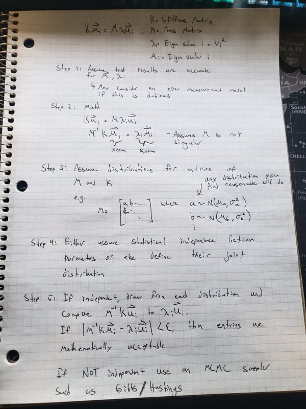
In what follows I'm assuming you are setting up your equation for K*u = lambda * M * u like shown
here. I'm also assuming that you what you're trying to do is use the test derived u / lambda values and back calculate acceptable K / M matrix entries.
If that's the case then the procedure below would kinda be what you would do with a few caveats. The first being that the solutions are not going to be unique, so you'll have an infinite number of acceptable combinations of entries that will produce the experimental results within epsilon. Some may be acceptable in a structural sense and others may not (unless you define the distributions to exclude these impossible combinations - see below). The second being that you'll definitely want to encode information that you know about the setup (e.g. impossible values or impossible combination of values) into your prior distributions for the various parameters - this can be difficult if we're assuming they covary as you need to define the full joint distribution.
Note: if you want to simulate effect of inputs on the matrix entries you can do that as well. For example, if entry a in Matrix M has a ~ N(u_a, var_a) then instead of assigning u_a directly you can assume u_a has its own distribution (e.g. u_a ~ N(beta_0 + beta_1 * input_1 + beta_2*input_2 + ..., var_input 1 + var_input 2 + ...)
On the other hand, if you have ample computing power you are free to just simulate from independent distributions, record those who produce results within epsilon and compare to your analytically derived results to see which of your simulations is closest. This is what the below protocol pretty much does (step 6 not shown is store and compare to your analytical results). You're likely to get lost in the high-dimensional space here though so defining the joint distribution and using MCMC is definitely the way to go IMHO.
As a note on efficiency I would probably avoid doing any inversions (computationally expensive) and would arrange my simulations / math accordingly. So my step 5 isn't how I would actually implement the thing but that's the concept.
Another note on efficiency is that if you can bound the various matrix entries, and establish incremental changes of interest, then you can randomly sample from the vector containing the bounds and all entries in-between. This will produce a large number of combinations, but infinitely less than assuming continuous distributions as I did in the procedure below.