Continue to Site

Eng-Tips is the largest engineering community on the Internet

Intelligent Work Forums for Engineering Professionals

  • Congratulations KootK on being selected by the Eng-Tips community for having the most helpful posts in the forums last week. Way to Go!

Nastran SOL 106 - Bi-/Tri-Linear Stress Strain result from Non-linear Material curve 1

Status
Not open for further replies.

jmarkus

Mechanical
Jul 11, 2001
377
Hi,

I have tried to simulate a tensile test of a dogbone specimen using SOL 106 in order to check my grasp of nonlinear simulation which I am still learning. Based on my results, I seem to be falling short in my understanding. The model consists of CQUAD4 shell elements, with one end of the specimen fully fixed and the other end subjected to a force only in the DOF 1 direction (aligned with the length of the specimen). I have LGDISP turned on. The material is defined by the stress-strain curve on the right side of the image below. The results of one of the elements with the highest stresses are shown as a stress-strain plot on the left side of the image. I was expecting the 2 curves to look similar, but the results from my simulation show 3 straight lines and not the same shape of the curve defined in the material. As well, the initial slope clearly doesn't match.
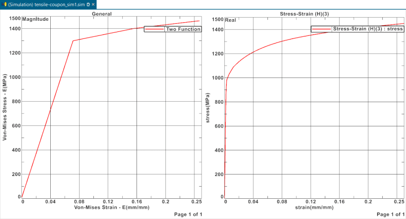
2024-03-31_220231_ihkamg.png


What could it be that I haven't taken into account (either in my understanding or in the simulation setup)?

Thanks,
Jeff
 
Replies continue below

Recommended for you

Why are you plotting von mises stress and strain?
You should be plotting axial stress and strain.
Show a deformation plot, and an axial stress plot.
You probably have over constrained the fixed end.
And first run SOL 101 with linear properties and be sure that works correctly
 
SW,

You are correct that I should be plotting axial stress and strain, I grabbed the default von-mises without thinking. However, this is a uniaxial tensile specimen, so the graphs look pretty much the same when plotted with axial stress/strains. I still only see a "multi-linear" curve instead of one with curvature like the material curve.

The fixed end has only the nodes at the very end of the specimen fixed. Would this be considered overconstrained?

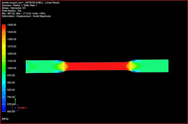
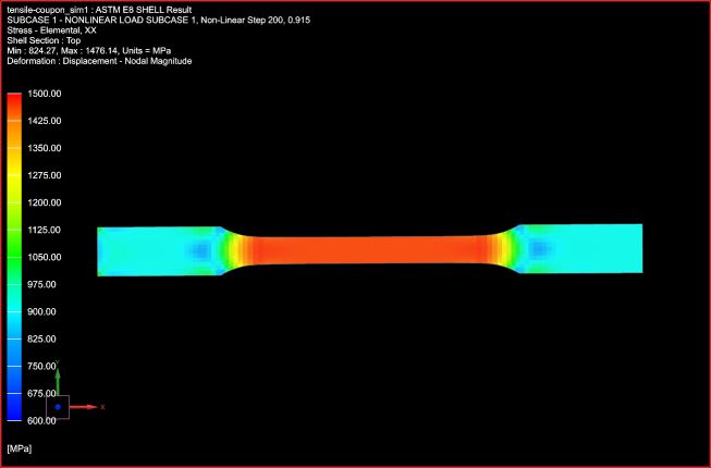
I ran SOL 101 and looking at the stress & strain contours, as well as the displacement looks ok to me. Since it is a linear analysis, I can't look at the stress or strain state across iterations like I do with the SOL 106. Below are contour plots from each simulation.

Linear:
2024-04-04_225836_gfglk5.jpg


Nonlinear:
2024-04-04_225908_ozw4qr.jpg


Is there a limitation in SOL 106 which I am not understanding?

Thanks,
Jeff
 
Hmmm, ok, the stress plots look ok.
Presumably you are plotting results from an element in the center of the gage section away from the radii. The nonlinear results should track the input stress-strain curve.
The only thing I can think of is some sort of load step convergence issue.
But I never much used sol 106 for nonlinear material analysis; greatly preferred Abaqus.
 
Your results plot looks like you're only getting output at a few load levels. And your first load level is already past the initial yield point, which is probably why the initial slope does not match. You need to obtain output at more steps as the load increases from zero to maximum to see the curve. The data points you have may be correct, but since you only have a few, you are not reproducing the entire curve.

You can get more steps in SOL 106 either by using multiple SUBCASEs and/or adding more increments to the NLPARM card. You should make sure you get at least some output in the linear range, and sufficient extra points near the knee of the curve if you want to reproduce that shape. SUBCASEs allow you to obtain output at any specified load level, while increments on the NLPARM card breaks the load of a given SUBCASE into NINC even steps.

For example, calculate the load to cause first yield: Py = Fty*b*t where b=specimen width and t = specimen thickness. Use this value of Py to decide how to break up the load into steps.

I would prefer the method of multiple SUBCASEs to have more control over load steps. Might be something like:

SUBCASE 1 = apply 50% Py
SUBCASE 2 = apply 75% Py
SUBCASE 3 = apply 100% Py
SUBCASE 4 = apply 120% Py
SUBCASE 5 = apply 130% Py
SUBCASE 6 = apply 150% Py

This ensures you will get output at these specific load levels (I purposely made them at unevenly spaced load levels to show what can be done). Within each SUBCASE, you can get one or more sets of output depending on your NLPARM settings, as follows:

NINC = number of increments the load in that SUBCASE is broken into. So, in SUBCASE 1 above, if NINC=5, then it will compute results at loads of 10,20,30,40, and 50% Py.

But, you will only get output at these "subincrements" if you have INTOUT=ALL on the NLPARM card. The default is INTOUT=NO, in which case you will only get the final output for that SUBCASE, i.e. 50% Py.

As SW suggested, you have to check that the results are converged as well. It will output the best it gets, but that does not necessarily mean that it has converged. I usually look in the .f06 output file for the message "CONVERGED" after each load increment to verify this.

I also would check to see how uniform the stress is across the width at the mid-length of the specimen. Look at the numerical values, not just the color contour plot. It should be uniform, but the stress concentrations near the ends drown out the mid-length stresses so they all appear one color in the contour plot, although the red range varies from 1425 to 1500. I'm guessing they are all 1500, but it would be prudent to confirm.
 
Tim,

I'm definitely getting somewhere now. Thanks to your suggestions, I split the load into subcases and made sure I was getting output throughout.

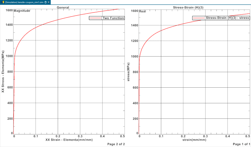
Here are my comparison plots:
2024-04-08_172740_yrcxd1.png


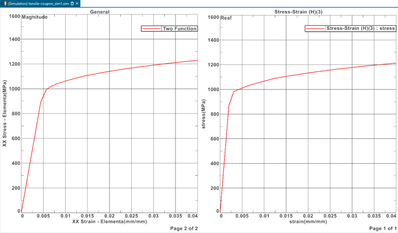
I still see some discrepancy in the initial slope (and the result near the end of the simulation). Here are plots zoomed into 0.04 strain. Any suggestions as to what is the missing piece of the puzzle?

2024-04-08_172934_a707zt.png


Thanks,
Jeff
 
The slope on the left (your results I guess) seems to be about 200,000 Mpa. The slope on the right (your input stress-strain curve I guess) seems to be about 480,000 Mpa. Which one is right? 200,000 Mpa seems about right for steel. Don't know what 480,000 Mpa would be.

In the plot on the right, exactly what types of stress and strain are being plotted? Are you sure that is a uniaxial tension stress-strain curve?

Just something else to check: did you try running it nonlinear material, but small displacements? (LGDISP turned off). As long as you have a nonlinear material defined, SOL 106 will consider the nonlinear material effects. LGDISP controls whether large or small displacements are considered, it has nothing to do with the material model.
 
Tim,

Good eye! I went back and looked at the material data I had entered for MATS1 and there was some typos in the first couple of points.

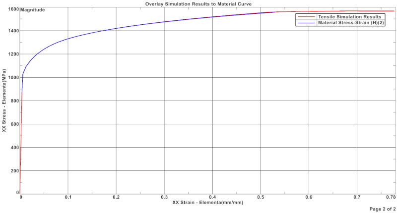
I corrected the data and re-ran the simulation, (and I learned how to overlay my results on the same graph) and now everything looks good!

2024-04-09_140613_g3kb4p.png


Thanks to both you and SW for helping me learn this! Now on to learn bigger and better things...I'm sure I'll be back for more help!
Jeff
 
Good, I'm glad you got it figured out. I also commend you for taking the time to completely understand a simple example before moving on to more complex problems. I shudder to think how many people are using these powerful tools without doing that...
 
Status
Not open for further replies.

Part and Inventory Search

Sponsor