Eng-Tips is the largest engineering community on the Internet

Intelligent Work Forums for Engineering Professionals

  • Congratulations waross on being selected by the Eng-Tips community for having the most helpful posts in the forums last week. Way to Go!

Python Solve Functions - Help For A Noobie 2

Status
Not open for further replies.

sticksandtriangles

Structural
Apr 7, 2015
468
US
sparked by the python coding discussion by Celt83, I am diving in and trying to solve instantaneous center of rotation problems with python.

The example problem I am trying to solve is outlined here:

The way I see this problem, there are (3) unknowns:
[ol 1]
[li]X location of the instantaneous center of rotation, [/li]
[/ol]
[ol 2]
[li]Y location of the instantaneous [/li]
[/ol]
[ol 3]
[li]and the Applied Loading that needs to be maxed out.[/li]
[/ol]

(sorry don't know how to fix the numbering above, fiddled for too damn long)

I also have (3) equations that need to equal 0
[ul]
[li]Sum of Forces in the X = 0[/li]
[/ul]
[ul]
[li] Sum of Forces in the Y = 0[/li]
[/ul]
[ul]
[li]Sum of Moments = 0 [/li]
[/ul]


Even in my "native coding language" matlab, this would be somewhat challenging to code, so I am sure it will be fun using this as a learning experience in python.

Anyways, python experts, do you have any suggestions on how to solve this? Should I explore symbolic notation within in python? Should I use a solve block that iterates through the (3) unknowns?

Any help or suggestions/starting points would be appreciated.

My base code that does the guess and check version of this is shown below:
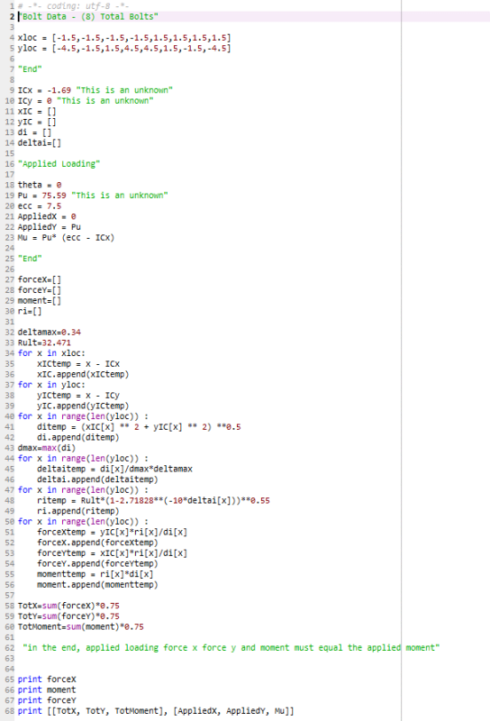
image_one_cr58iv.png

The final print shows the comparison of applied loading verse resist force.
image_2_fuboii.png


S&T
 
Replies continue below

Recommended for you

The Scipy library has several solver functions that will do what you want.

Examples can be found in my xlScipy3 spreadsheet, which can be downloaded from:

The spreadsheet calls the Python functions from Excel using xlwings, but if you prefer to work directly with Python the Python code is included in the download.

For solvers with more than one unknown see the Solvers2 sheet, which use the Scipy.Optimize minimize function. You need to write a function that returns the difference between calculated and target values for given inputs, with output as a Numpy array, and the minimize function will adjust the inputs to minimize the differences.


Doug Jenkins
Interactive Design Services
 
IDS, thank you.

I am digging into these spreadsheets now and will check in later (got scipy downloaded).
Feel a little overwhelmed currently [spin2], lots of learning to ensue...

S&T
 
Let us know how you go.

To use Scipy you will also need Numpy, but they are both pretty well indispensable for engineering work with Python.

As an example of what you can do with Numpy, using the xloc list from your code:

Python:
import numpy as np
…
# Convert xloc to a Numpy array
xloc = np.array(xloc)
ICX = -1.69
# Subtract ICX from all xloc values in one operation
xIC = xloc - ICX

Doug Jenkins
Interactive Design Services
 
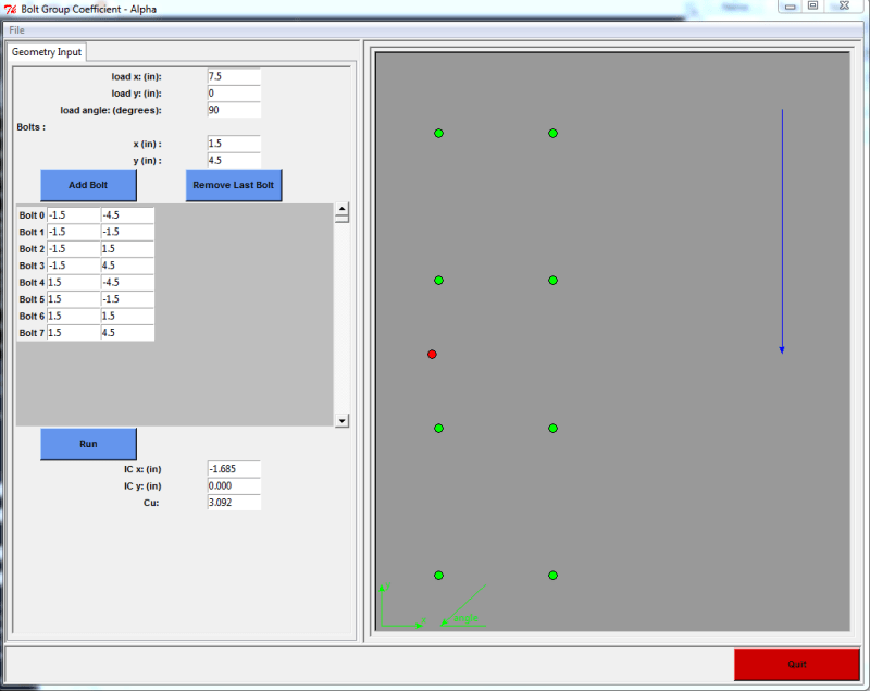
hmm learned something new hadn't ever looked into Scipy for this, here's my code below which seems to check out:
It is pretty sensitive to where the initial IC coordinates are assumed to be

As IDS notes you can condense a lot of this down to single line steps using numpy arrays, I kept the bulk of it as native python lists and broken up into the calculation steps.

Python:
from __future__ import division
import math as m
import scipy.optimize as sci

def ic_check(IC,xloc,yloc, ecc, theta):
    num_bolts = len(xloc)
    
    deltamax = 0.34
    Rult = 32.471
    
    ICx = IC[0]
    ICy = IC[1]
    xIC = []
    yIC = []
    di = []
    deltai = []
    ri = []
    
    fx = []
    fy = []
    moment = []
    
    for x in xloc:
        xICtemp = x - ICx
        xIC.append(xICtemp)
        
    for y in yloc:
        yICtemp = y - ICy
        yIC.append(yICtemp)
    
    i=0
    for i in range(num_bolts):
        ditemp = m.sqrt((xIC[i]*xIC[i])+(yIC[i]*yIC[i]))
        di.append(ditemp)
    
    dmax = max(di)
    
    i=0
    for i in range(num_bolts):
        deltaitemp = (di[i]/dmax)*deltamax
        deltai.append(deltaitemp)
        
    i=0
    for i in range(num_bolts):
        ritemp = Rult*m.pow(1-m.pow(m.e,-10.0*deltai[i]),0.55)
        ri.append(ritemp)
        
    i=0
    for i in range(num_bolts):    
        fxtemp = (yIC[i]*ri[i])/di[i]
        fx.append(fxtemp)
        
    i=0
    for i in range(num_bolts):     
        fytemp = (xIC[i]*ri[i])/di[i]
        fy.append(fytemp)
        
    i=0
    for i in range(num_bolts):    
        momenttemp = ri[i]*di[i]
        moment.append(momenttemp)
    
    totX = sum(fx)*0.75
    totY = sum(fy)*0.75
    totM = sum(moment)*0.75
    
    Pu_force = m.sqrt((totX*totX) + (totY*totY))
    
    Pu_moment = totM / (ecc - ICx*m.cos(m.radians(theta)) - ICy*m.sin(m.radians(theta)))
    
    res1 = [totX, totY, totM]
    
    res2 = [Pu_force, Pu_moment]
    
    return res1, res2
    
def ic_optimize(IC,xloc,yloc,ecc,theta):
    
    res1, res2 = ic_check(IC,xloc,yloc,ecc,theta)
    
    res = res2[0] - res2[1]
    
    return abs(res)
    
xloc = [-1.5,-1.5,-1.5,-1.5,1.5,1.5,1.5,1.5]
yloc = [-4.5,-1.5,1.5,4.5,4.5,1.5,-1.5,-4.5]

ICx = -1.69
ICy = 0.0
IC = [ICx,ICy]
theta = 0.0
ecc = 7.5
res1, res2 = ic_check(IC,xloc,yloc,ecc,theta)

test2 = ic_optimize(IC,xloc,yloc,ecc,theta)

test = sci.minimize(ic_optimize,IC,(xloc,yloc,ecc,theta), tol=1e-6)

IC_new = [test.x[0],test.x[1]]

res3, res4 = ic_check(IC_new,xloc,yloc,ecc,theta)

Open Source Structural Applications:
 
I improved the results slightly by also back checking sum Fx and sum Fy in my optimization function:
It is still very sensitive to the initial IC coordinate guess.

There is a great article on AISC for this by G. Donald Brandt from 2nd quarter 1982:
Python:
def ic_optimize(IC,xloc,yloc,ecc,theta):
    
    res1, res2, check = ic_check(IC,xloc,yloc,ecc,theta)
    
    res = res2[0] - res2[1]
    
    px = res2[0]*m.sin(m.radians(theta))
    py = res2[0]*m.cos(m.radians(theta))
    
    fx = px + res1[0]
    fy = py - res1[1]
    
    res_magnitude = m.sqrt(res*res+fx*fx+fy*fy)
    
    return res_magnitude

Open Source Structural Applications:
 
Brandt's Method is much more reliable:

Python:
from __future__ import division
import math as m
import scipy.optimize as sci

def ic_check(IC,xloc,yloc, ecc, theta):
    num_bolts = len(xloc)
    
    deltamax = 0.34
    Rult = 32.471
    
    ICx = IC[0]
    ICy = IC[1]
    xIC = []
    yIC = []
    di = []
    deltai = []
    ri = []
    
    fx = []
    fy = []
    moment = []
    
    for x in xloc:
        xICtemp = x - ICx
        xIC.append(xICtemp)
        
    for y in yloc:
        yICtemp = y - ICy
        yIC.append(yICtemp)
    
    i=0
    for i in range(num_bolts):
        ditemp = m.sqrt((xIC[i]*xIC[i])+(yIC[i]*yIC[i]))
        di.append(ditemp)
    
    dmax = max(di)
    
    i=0
    for i in range(num_bolts):
        deltaitemp = (di[i]/dmax)*deltamax
        deltai.append(deltaitemp)
        
    i=0
    for i in range(num_bolts):
        ritemp = Rult*m.pow(1-m.pow(m.e,-10.0*deltai[i]),0.55)
        ri.append(ritemp)
        
    i=0
    for i in range(num_bolts):    
        fxtemp = (yIC[i]*ri[i])/di[i]
        fx.append(fxtemp)
        
    i=0
    for i in range(num_bolts):     
        fytemp = (xIC[i]*ri[i])/di[i]
        fy.append(fytemp)
        
    i=0
    for i in range(num_bolts):    
        momenttemp = ri[i]*di[i]
        moment.append(momenttemp)
    
    totX = sum(fx)*0.75
    totY = sum(fy)*0.75
    totM = sum(moment)*0.75
    
    Pu_force = m.sqrt((totX*totX) + (totY*totY))
    
    Pu_moment = totM / (ecc - ICx*m.cos(m.radians(theta)) - ICy*m.sin(m.radians(theta)))
    
    res1 = [totX, totY, totM]
    
    res2 = [Pu_force, Pu_moment]
    
    check_output = [xIC,yIC,di,deltai,ri,fx,fy]
    
    return res1, res2, check_output
    
def ic_optimize(IC,xloc,yloc,ecc,theta):
    
    res1, res2, check = ic_check(IC,xloc,yloc,ecc,theta)
    
    res = res2[0] - res2[1]
    
    px = res2[0]*m.sin(m.radians(theta))
    py = res2[0]*m.cos(m.radians(theta))
    
    fx = px - res1[0]
    fy = py - res1[1]
    
    res_magnitude = m.sqrt(res*res+fx*fx+fy*fy)
    
    return res_magnitude

def ic_brandt(IC, xloc, yloc, Mp):
    num_bolts = len(xloc)
    
    deltamax = 0.34
 
    ICx = IC[0]
    ICy = IC[1]
    xIC = []
    yIC = []
    di = []
    deltai = []
    ri = []
    
    fx = []
    fy = []
    moment = []
    
    for x in xloc:
        xICtemp = x - ICx
        xIC.append(xICtemp)
        
    for y in yloc:
        yICtemp = y - ICy
        yIC.append(yICtemp)
    
    i=0
    for i in range(num_bolts):
        ditemp = m.sqrt((xIC[i]*xIC[i])+(yIC[i]*yIC[i]))
        di.append(ditemp)
    
    dmax = max(di)
    
    i=0
    for i in range(num_bolts):
        deltaitemp = (di[i]/dmax)*deltamax
        deltai.append(deltaitemp)
        
    i=0
    for i in range(num_bolts):
        ritemp = m.pow(1-m.pow(m.e,-10.0*deltai[i]),0.55)
        ri.append(ritemp)
        
    i=0
    for i in range(num_bolts):    
        fxtemp = -1*(yIC[i]*ri[i])/di[i]
        fx.append(fxtemp)
        
    i=0
    for i in range(num_bolts):     
        fytemp = (xIC[i]*ri[i])/di[i]
        fy.append(fytemp)
        
    i=0
    for i in range(num_bolts):    
        momenttemp = ri[i]*di[i]
        moment.append(momenttemp)
    
    Mi = sum(moment)
    Rult = -1*Mp/Mi
    
    Rx = sum(fx) * Rult
    Ry = sum(fy) * Rult
    
    
    table = [xIC, yIC, di, deltai, ri, moment, fx, fy]
    
    return Rx, Ry, Mi, table
    
def brandt(xloc, yloc, P_xloc, P_yloc, P_angle):
    # Bolt Group Instantaneous Center using method by G. Donald Brandt
    # Rapid Determiniation of Ultimate Strength Of Eccentrically Loaded Bolt Groups
    # AISC Journal 1982 2nd Quarter
    
    detailed_output = []
    
    num_bolts = len(xloc)
    
    n = num_bolts
    
    detailed_output.append(num_bolts)
    
    #Bolt Group Centroid
    if len(xloc)<3:
        anchor_x_bar = (xloc[0]+xloc[1])/2.00
        anchor_y_bar = (yloc[0]+yloc[1])/2.00
    
    else:
        j=0
        x_tot=0
        y_tot=0
        
        for i in xloc:
            x_tot = x_tot+xloc[j]
            y_tot = y_tot+yloc[j]    
            j+=1
        
        anchor_x_bar = x_tot/len(xloc)
        anchor_y_bar = y_tot/len(yloc)
     
    cg_anchors = [anchor_x_bar, anchor_y_bar]
    detailed_output.append(cg_anchors)
    
    # J - Polar Moment of Inertial of Bolt Group
    # sum(x^2+y^2)
    sum_x_square = 0
    sum_y_square = 0
    
    i=0
    for i in range(num_bolts):
        sum_x_square = sum_x_square + (xloc[i]-anchor_x_bar)**2
        sum_y_square = sum_y_square + (yloc[i]-anchor_y_bar)**2
    
    J = sum_x_square + sum_y_square
    detailed_output.append(['J',J])
    
    Px = -1*m.cos(m.radians(P_angle))
    Py = -1*m.sin(m.radians(P_angle))
    
    detailed_output.append([Px,Py])
    
    Mo = (-1*Px*(P_yloc-anchor_y_bar))+(Py*(P_xloc-anchor_x_bar))
    
    detailed_output.append(Mo)
    
    ax = (-1*Py*J) / (n * Mo)
    ay = (Px*J) / (n*Mo)
    
    detailed_output.append([ax,ay])
    
    Mp = (-1*Px*(P_yloc-anchor_y_bar-ay))+(Py*(P_xloc-anchor_x_bar-ax))
    
    detailed_output.append(Mp)
    
    IC_initial = [anchor_x_bar+ax,anchor_y_bar+ay]
    
    Rx, Ry, Mi, table = ic_brandt(IC_initial,xloc,yloc, Mp)
    
    detailed_output.append([Rx, Ry, Mi, table,"First IC pass"])
    
    fxx = Px + Rx
    fyy = Py + Ry
    F = m.sqrt(fxx*fxx+fyy*fyy)
    
    detailed_output.append([fxx,fyy,F,"F"])
    
    ax_new = (-1*fyy*J)/(n*Mo)
    ay_new = (fxx*J) / (n*Mo)
    
    detailed_output.append(["ax",ax_new,"ay",ay_new])
    
    IC_new = IC_initial  
    
    count = 0
    iterations = 0
    while count<1000:
        
        IC_new = [IC_new[0]+ax_new,IC_new[1]+ay_new]
        Mp_new = (-1*Px*(P_yloc-IC_new[1]))+(Py*(P_xloc-IC_new[0]))
        
        Rx, Ry, Mi, table = ic_brandt(IC_new,xloc,yloc, Mp_new)
        
        fxx = Px + Rx
        fyy = Py + Ry
        F = m.sqrt(fxx*fxx+fyy*fyy)
        
        ax_new = (-1*fyy*J)/(n*Mo)
        ay_new = (fxx*J) / (n*Mo)
        
        if F <= 0.00001:
            iterations = count
            count = 1000          
            solution = 'yes'
        else:        
            count +=1
            solution = 'no'
    
    detailed_output.append([fxx,fyy,F])        
    detailed_output.append(IC_new)
    detailed_output.append([solution,iterations,count])
    
    detailed_output.append([Rx, Ry, Mi, table])


    Cu = abs(Mi/Mp_new)
    
    detailed_output.append([Mi,Mp_new,Cu])
    
    return detailed_output, IC_new, Cu

# From Scratch Method Testing Zone    
xloc = [-1.5,-1.5,-1.5,-1.5,1.5,1.5,1.5,1.5]
yloc = [-4.5,-1.5,1.5,4.5,4.5,1.5,-1.5,-4.5]

#Center of Anchor Group
if len(xloc)<3:
    anchor_x_bar = (xloc[0]+xloc[1])/2.00
    anchor_y_bar = (yloc[0]+yloc[1])/2.00

else:
    j=0
    x_tot=0
    y_tot=0
    
    for i in xloc:
        x_tot = x_tot+xloc[j]
        y_tot = y_tot+yloc[j]    
        j+=1
    
    anchor_x_bar = x_tot/len(xloc)
    anchor_y_bar = y_tot/len(yloc)

ICx = anchor_x_bar
ICy = anchor_y_bar
IC = [ICx,ICy]
theta = 0
ecc = 4
res1, res2, check1 = ic_check(IC,xloc,yloc,ecc,theta)

test2 = ic_optimize(IC,xloc,yloc,ecc,theta)

test = sci.minimize(ic_optimize,IC,(xloc,yloc,ecc,theta),method='Nelder-Mead', tol=1e-6)

IC_new = [test.x[0],test.x[1]]

res3, res4, check2 = ic_check(IC_new,xloc,yloc,ecc,theta)
    
C = res4[0]/(0.75*32.471)   

# Brandt's Method Testing Zone
# angle is positive counter-clockwise and measured from 0 pointing to the right
# anchor and P coordinates are global
x_b = [-1.5,-1.5,-1.5,-1.5,1.5,1.5,1.5,1.5]
y_b = [-4.5,-1.5,1.5,4.5,4.5,1.5,-1.5,-4.5]
P_xloc = 7
P_yloc = 0
P_angle = 90

brandt = brandt(x_b, y_b, P_xloc, P_yloc, P_angle)

Open Source Structural Applications:
 
thank you a ton Celt.

A few questions for you as I am trying to parse this code.

What does return do in python:
Python:
        momenttemp = ri[i]*di[i]
        moment.append(momenttemp)
    
    totX = sum(fx)*0.75
    totY = sum(fy)*0.75
    totM = sum(moment)*0.75
    
    Pu_force = m.sqrt((totX*totX) + (totY*totY))
    
    Pu_moment = totM / (ecc - ICx*m.cos(m.radians(theta)) - ICy*m.sin(m.radians(theta)))
    
    res1 = [totX, totY, totM]
    
    res2 = [Pu_force, Pu_moment]
    
    check_output = [xIC,yIC,di,deltai,ri,fx,fy]
    
    [b][u]return[/u][/b] res1, res2, check_output

It looks like the program now knows the variables res1, res2, and check_output after the function is performed. Is this correct?

Could the (2) functions you have created be combined into one function? It looks like ic_optomize just builds on results from ic_check? The way I am interrupting this, res_magnitude (the final output from ic_optomize) could be programmed into ic_check.

Could the minimize function then be run ic_check in this case? Or does the function that is being minimized only allowed to have (1) output?


S&T
 
i will also dig into the Brandt method when I get back to the office to login into AISC.

Looks like nice method for quick convergence.

S&T
 
The return line at the end of the function specifies what variable or value can be assigned as the function result to be used globally for further operations.

I have limited knowledge of how to properly use the scipy.optimize.minimize function but it seemed to want one result to check against, i also found that if the result was negative it would keep going negative rather than adjust to start returning back closer to 0.

Open Source Structural Applications:
 
Cool stuff Celt! Digging into the GUI stuff this weekend once I get some free time.

S&T
 
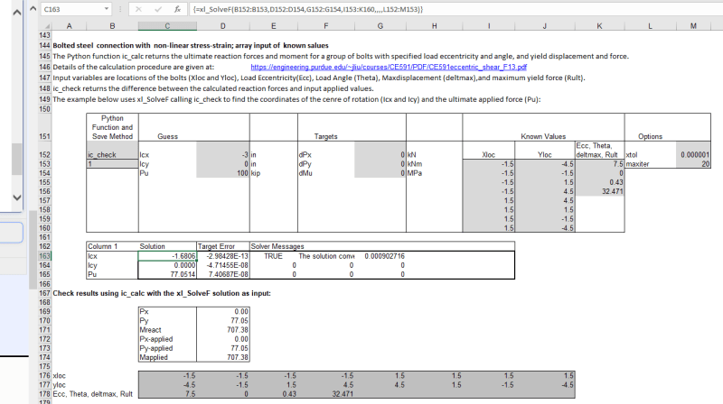
I have now set this up to run using the Scipy.optimize root function:

Python:
def xlic_calc(IC, xloc, yloc, vals):
    ecc =vals[0]
    theta = np.radians(vals[1])
    deltamax = vals[2]
    Rult = vals[3]
    num_bolts = len(xloc)
    
    ICx = IC[0]
    ICy = IC[1]
    Pu = IC[2]
    Pux = Pu * np.sin(theta)
    Puy = Pu * np.cos(theta)
    Mu = Pu * (ecc-ICx*np.cos(theta)-ICy*np.sin(theta))
    xIC = []
    yIC = []
    di = []
    deltai = []
    ri = []
    
    fx = []
    fy = []
    moment = []
    
    for x in xloc:
        xICtemp = x - ICx
        xIC.append(xICtemp)
        
    for y in yloc:
        yICtemp = y - ICy
        yIC.append(yICtemp)
    
    i=0
    for i in range(num_bolts):
        ditemp = np.sqrt((xIC[i]*xIC[i])+(yIC[i]*yIC[i]))
        di.append(ditemp)
    
    dmax = max(di)
    
    i=0
    for i in range(num_bolts):
        deltaitemp = (di[i]/dmax)*deltamax
        deltai.append(deltaitemp)
    
        ritemp = Rult*(1-np.e**(-10.0*deltai[i]))**0.55
        ri.append(ritemp)
                    
        fxtemp = (yIC[i]*ri[i])/di[i]
        fx.append(fxtemp)
             
        fytemp = (xIC[i]*ri[i])/di[i]
        fy.append(fytemp)
          
        momenttemp = ri[i]*di[i]
        moment.append(momenttemp)
    
    totX = sum(fx)*0.75
    totY = sum(fy)*0.75
    totM = sum(moment)*0.75
    
    return [totX, totY, totM, Pux, Puy, Mu]

It's set up to be called from Excel using xlwings, but you can also call direct from Python:

>>> res = sopt.root(ic_check, x0, vals2)
>>> res.x
array([-1.68496865e+00, 4.01869965e-16, 7.53006559e+01])

Doug Jenkins
Interactive Design Services
 
continued:
Inputs are:
x0, the initial guess: [-3, 0,100]
vals2: [[target vals],[[Xloc],[Yloc],[knowns]]]

[target vals] = [0,0,0]
[knowns] = [Eccentricity, Theta, deltamax,Rult]

I didn't have any problem with sensitivity to the initial guess values, and it works very fast with the default solver. Several of the other solvers work very slowly, or not at all.

I will post the Excel version in the next few days. Here's what it looks like:

Scipy-solve_l9l10n.png


Doug Jenkins
Interactive Design Services
 
Part 3.

The ic_check function, which is the one you call from sopt.root:

Python:
def ic_check(IC, vals):   
    xloc = vals[1][0]
    yloc  = vals[1][1]
    vals2 =vals[1][2]
    
    res1 = xlic_calc(IC,xloc, yloc, vals2)
    
    totX = res1[0]
    totY = res1[1]
    totM = res1[2]
            
    Pu =IC[2]
    Pux = res1[3]
    Puy = res1[4]
    Mu = res1[5]
    
    res3 = [totX-Pux, totY-Puy, totM-Mu]
    
    return res3

Doug Jenkins
Interactive Design Services
 
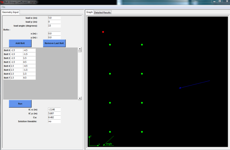
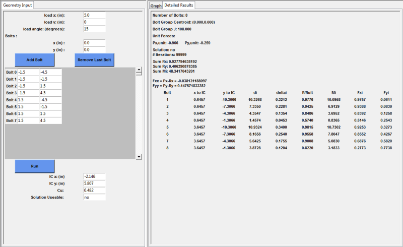
It was a tolerance issue certain bolt and load configurations don't converge beyond a certain precision. I added the ability to control the tolerance.

the 8 bolt group needed a tolerance of 0.00001
a 3 bolt group (0,0) (0,3) (0,6) load at (5,3) angle: 15 needed a tolerance of 0.1 on my end

I'm sure the scipy module may have something built in to handle these odd conditions.

Open Source Structural Applications:
 
Status
Not open for further replies.

Part and Inventory Search

Sponsor

Back
Top