Continue to Site

Eng-Tips is the largest engineering community on the Internet

Intelligent Work Forums for Engineering Professionals

  • Congratulations KootK on being selected by the Eng-Tips community for having the most helpful posts in the forums last week. Way to Go!

Shaft Critical Speed Calculator Based on Melvin prohls Method 2

Status
Not open for further replies.

Basit Shafi

Mechanical
May 23, 2023
11
Hi,

I am trying to program a critical speed calculator , the prime purpose is to calculate the first critical speed as accurately as possible by taking into account the gyroscopic effects and bearing stiffness , It should also estimate to 2nd and third critical speeds in some instances where a preliminary information for a detailed rotordynamic analysis is required.

I have found a method mentioned in the paper "
There is no example given for the gyroscopic effect just an explanation of how to do it. Has anyone programmed this calculator or something similar .

I have found an article where @ELECTRICPETE talks about the leisley fielding book, does it include this method?


Thank you

AbdAlBasit
 
Replies continue below

Recommended for you

No I haven't. Wow what a paper.

It says "The last tw~ columns on the form, Table 1, hav~ been added so
that the effect of the mass moment of inerti~ of the disks may be
incorporat.ed into the. calculation. The heading-oi_ column 18
applies t.o tll.e rotatit}g case. I"

more or less, OCR being less than perfect. This is right at the end , after equation 50

So it looks like you have to use the last two columns in the table.

I must admit I'm a bit wary of that whole idea, it would be dependent on the actual angular velocity in bending and I would hazard a guess it might be non linear on displacement. I think the gyroscopic effect would stiffen the system (ie raise the first mode). Odd for an inertia related term.

Cheers

Greg Locock


New here? Try reading these, they might help FAQ731-376
 
The Prohl method as I understand is also called the Mykelstad Prohl method or simply the "transfer matrix" method.

I'm pretty sure that book you mentioned does have a lot of details about it. It's not accessible to me at the moment, I'll double check tonight if I remember.

I used that book and maybe a few others to program the transfer matrix method into an excel spreadsheet with vba. The numerical part was the easier part, the harder part was trying to create a useable interface. I ended up with an interface which is very useable for myself but might take some getting used to for others.

I built a website about my spreadsheet/program although the website is not online... it's just a directory of html files and related excel files that they link to (stored locally on my flash drive). I'm not sure I know how to make it accessible (nor if anyone would feel comfortable running vba code from an anonymous internet stranger) so let me post two of the html pages (converted to pdf) that are related:
[ol 1]
[li]The first file is probably of more interest. It has a filename xfmatdiscussion.pdf and it goes through the math model of the transfer matrix method used in gory detail... I tried to include every equation, assumption and convention that I made so to my thinking it has everything needed to build the program yourself. In the middle of the 3rd page it talks about the parameter J used in the mass matrix which captures both the "in-plane tilting disk effects" which reduce the natural frequencies during impact/bump test of a stationary rotor and the gyroscopic effects which increase the natural frequencies of a rotating rotor. In my terminology, the parameter J is some combination of polar moment of inertia Ip and diametral moment of inertia Id depending on which of three "gyroscopic options" is selected (critical speed option models rotating rotor, bump test option models stationary rotor, and a simple/point mass option has no-tilting-disk effects at all). The formulas used for Ip, Id are included. By the way what I refer to as "in-plane tilting disk effects" are more commonly called "rotary inertia" effects, but I hate that rotating inertia terminology in the context of rotating equipment because the rotary they're referring to has nothing to do with the rotation of the equipment (it's associated with change in slope of the axis of disk sections associated with the rotor). These bump test tilting disk effects are in-plane tilting disk effects because the y direction model depends only on tilting in the y-z plane, in contrast to gryoscopic where y direction behavior also depends on tilting in the x-z plane.[/li]
[li]I also have attached a second file titled RotoSolveDemo.pdf which shows the results of my spreadsheet applied to various scenarios (generally starting small and working more complex) as a means of validation (it validates that the spreadsheet gives answers matching solutions calculated other ways for the cases examined). Of interest, there is a section VII at the end which shows what happens when you apply the three different gyroscopic options to an example overhung rotor... maybe that explains better what is going on with those three "gryroscopic options".[/li]
[/ol]
Both of the above files include a lot of "links" to files that won't work for you. If you want me to upload the files associated with any of those links, let me know.

PS there are some limitations of the transfer matrix method.
[ul]
[li]First, in the way I have implemented it, it only works for axisymmetric support (bearing and support parameters are the same in the x and y directions). I understand there's a way to build two linked transfer matrix models to fix that, but I never bothered.[/li]
[li]Second, it can model the rotor in detail and it can model stationary stiffnesses, but it can NOT model stationary masses like for example if there is mass associated with the bearing pedestal. If you were trying to model a vertical motor that would be quite a handicap because movement of stationary masses (the stator) can play a big role. I'm pretty sure it is a limitation of the method which cannot be overcome because I have seen other implementations that don't allow to model stationary masses. That leads me to one more thing... [/li]
[/ul]
The second limitation above leads me to mention a prominent open source rotordynamics package ROSS (programmed in python) which I believe uses the transfer matrix method. There is some info about it at these links
[ul]
[li][/li]
[li][/li]
[li][/li]
[/ul]
That ROSS program in general doesn't look particularly user friendly (I think you have to model the rotor by setting up text files rather than using a GUI). They call it a "finite element" method, which is too general a term in this context (it could mean a lot of things). If they did it the way Maurice Adams does in his book, they would build one huge K matrix, one huge M matrix and one huge C or G matrix to capture the whole model and solve it as an eigenvalue/eigenvector problem. If they used Adam's large matrix approach they could easily include stationary masses. But ROSS does not seem to have any provision to model stationary masses. That limitation leads me to believe they are using the transfer matrix method (although I haven't looked at the code)
 
As described by others, If the main mass is a disc sort of in the middle of the shaft it won't bend/tip during 1st mode vibration so gyroscopic stiffening effects will be small.

Do you have a specific application?
If the the first mode was raised 5% by gyroscopic effect would it pose a problem?
 
@Tmoose One silly example where it would be important is a shaft with a flywheel outboard of the bearings.

@ep am I right that the gyroscopic effect stiffens the system?

Your comment about different bearing stiffnesses in the two planes set off alarm bells in my head but I am very rusty on this stuff, can that cause half speed whirl?

Cheers

Greg Locock


New here? Try reading these, they might help FAQ731-376
 
@GregLocock , I know that bit , I just wanted to know how to add the moments properly which I have done now. Thank you for your response.


@electricpete The paper that I have attached has the same essence as that of the transfer matrix method ( the initial conditions lay a chain reaction of effects along different sections) , in fact this paper was the beginning of the transfer matrix method. At the moment given the situation right now and given the program I need to put it this rotordynamic program into needs a spreadsheet-type layout and this paper does it well . The only confusion for me is that, the illustration in the paper doesn't cover the addition of stiffness and a case where the calculations start from the overhand on the left end side .


I need to add stiffness to the system so that the deflections at the bearings wont be zero. Also , like I said The illustration of the paper is a shaft between bearings and an overhang on the right . I need a case where it starts with an overhang on the left and goes to the middle section then overhang on the right with the bearing stiffnesses added. I need someone to help me verify if I am doing the right thing .


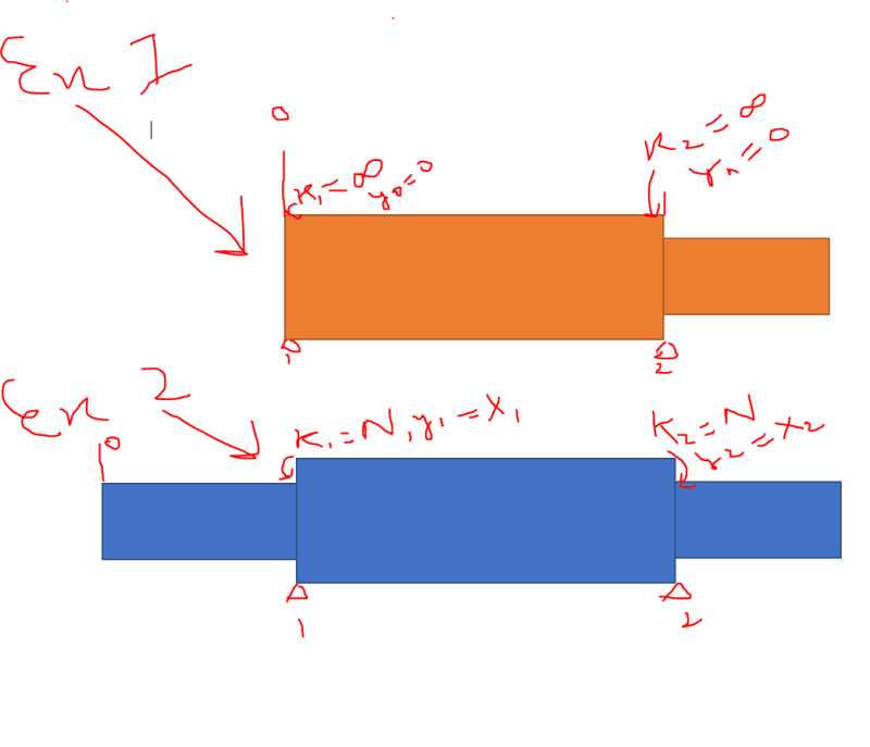
I have attached a picture where the case 1 in orange represents the example in the paper , station 0 being bearings itself, where stiffness is infinite ( simply supported case) ,

But What I want is the picture in blue where there station 0 is the free end and stiffnesses are finite and hence deflections are present at bearing supports.I don't know if anyone could help to go through the paper and produce an example in blue.

Rotor_trv8oe.png
 
I don't have time to go through the paper at the moment. I can refer to my own "paper" xfmatdiscussion.pdf linked above to show how the bearing is treated.

Referring to xfmatdiscussion.pdf very first figure shows Sleft, Smiddle, Sright.
Smiddle = Pi * Sleft
Sright = Fi * Smiddle
Sright = Fi * Pi * Sleft

If you have a bearing attached to node i, then it affects the relation between Sleft and Smiddle and so its influence will show in the "point matrix" Pi. Further into the paper you see the definition of the point matrix Pi and indeed it includes a term -Kbrg in the lower left hand corner. That position must be considered in the context of my state matrix which is defined as S = [Y, T, M, V] ' When evaluating Smiddle = Pi * Sleft, that -Kbrg in the lower left position tells us that the last index of Smiddle (i.e. Vmiddle) will include a summed contribution of four terms the last of which is -Kbrg times the first index of Sleft (i.e. Yleft). So the shear Vmiddle includes an additive term -Kbrg * xleft which accounts for the displacement-dependent force applied by the bearing to the rotor. It also include an additive contributioin from 1*Vleft owing to the coefficient 1 located in the lower right of the P matrix. So Vmiddle = Vleft - Kbrg*x... which means that as we traverse the rotor from left to right, the shear changes every time there is a bearing, as expected. There are also changes due to mass acceleration but those would be captured elsewhere (they're in the field matrix assuming distributed mass calculation).

Everything needs to be a consistent set of conventions. In the end the transformation from Sleft to Smiddle and Smiddle to Sright should make sense using first principles. I don’t know if that helps but that’s all I’ve got now...

Actually if it helps I do have the analytical part of my vba code (below) segregated from the input/output part, and the terminology is consistent with xfmatdiscussion.pdf. The routine findstationmatrix finds the 4x4 station matrix (Si = Fi*Pi) for the ith rotor section (station). The form of that matrix should match what was stated in xfmatdiscussion.pdf. the function findobjective function accepts a test guess wt for the resonant frequency and assembles all the individual station matrices to find the transformation from the left side boundary conditions to the right side boundary condition and uses that information to generate a scalar output which would be zero if-and-only-if plugging in the boundary conditions at the LHS results in the correct boundary conditions at the rhs. different values of wt are tried using bisection algorithm to find the ones that satisfy the boundary conditions. mequals and lmult are user-defined vba functions representing matrix assignment and multiplication in the traditional way that I saw a need to program myself for some reason (as I recall, I had some problem getting the worksheet matrix functions to work within vba). I can guarantee the code works (it's the same used in my validation examples), but I can't guarantee that it's striaghtforward to translate without the benefit of the other vba routines and the input variables that are embedded in the spreadsheet itself (there may be a few calculations embedded in the spreadsheet too)
Code:
[tt]Option Explicit
Option Base 1
' Public calledfromplotmodeshape As Boolean 'findobjective can be called from two procedures
' deleted as public variable and move to a calling parameter
Public leftstate(4) As Double ' passed from findobjective to plotmodeshape

Function findstationmatrix(index As Integer, wt As Double, brgmult As Double)
' index tells which element we are accessing
' wt is trial value of w at which we are evaluating the stationmatrx
' brgmult is bearing stiffness multiplier
Dim tempstationmatrix(4, 4) As Double ' temporary placeholder for the output findstationmatrix
  ' can't assign directly to findstationmatrix() since would look like a function call
Dim Kbrg As Double ' temporary (prettier) name for pdata(index).bearingstiffness*Kmult
Dim J As Double ' temporary (prettier) name for pdata(index).jp
Dim ei As Double   ' temporary (prettier) name for sdata(index).ei


Kbrg = pdata(index).brgstiffness * brgmult
J = pdata(index).jp  ' note inclgryo option already factored in within getinputandinitialize module
ei = sdata(index).ei

If Worksheets("main").Range("lumpedmasscalc").Value = True Then
  ' LUMPED MASS CALC HERE
  Dim L As Double
  Dim m As Double
  L = sdata(index).length
  m = pdata(index).mpoint
  tempstationmatrix(1, 1) = 1 + L ^ 3 * (m * wt ^ 2 - Kbrg) / (6 * ei)
  tempstationmatrix(1, 2) = L + L ^ 2 * J * wt ^ 2 / (2 * ei)
  tempstationmatrix(1, 3) = L ^ 2 / (2 * ei)
  tempstationmatrix(1, 4) = L ^ 3 / (6 * ei)
  
  tempstationmatrix(2, 1) = L ^ 2 * (m * wt ^ 2 - Kbrg) / (2 * ei)
  tempstationmatrix(2, 2) = 1 + L * J * wt ^ 2 / ei
  tempstationmatrix(2, 3) = L / ei
  tempstationmatrix(2, 4) = L ^ 2 / (2 * ei)
  
  tempstationmatrix(3, 1) = L * (m * wt ^ 2 - Kbrg)
  tempstationmatrix(3, 2) = J * wt ^ 2
  tempstationmatrix(3, 3) = 1
  tempstationmatrix(3, 4) = L
  
  tempstationmatrix(4, 1) = m * wt ^ 2 - Kbrg
  tempstationmatrix(4, 2) = 0
  tempstationmatrix(4, 3) = 0
  tempstationmatrix(4, 4) = 1

Else
  ' DISTRIBUTED MASS CALC HERE
  Dim k As Double ' kappa
  Dim kfourth As Double  'k^4 will be handy value to store
  Dim kL As Double ' k * Length of section
  Dim C0 As Double
  Dim S1 As Double
  Dim C2 As Double
  Dim S3 As Double
  k = (wt ^ 2 * sdata(index).RhoAoverEI) ^ 0.25
  kfourth = k ^ 4
  kL = k * sdata(index).length
  C0 = (Cos(kL) + Application.Cosh(kL)) / 2
  S1 = (Sin(kL) + Application.Sinh(kL)) / 2 / k
  C2 = (-Cos(kL) + Application.Cosh(kL)) / 2 / k ^ 2
  S3 = (-Sin(kL) + Application.Sinh(kL)) / 2 / k ^ 3
  
  tempstationmatrix(1, 1) = C0 - 1 / ei * S3 * Kbrg
  tempstationmatrix(1, 2) = S1 + 1 / ei * C2 * J * wt ^ 2
  tempstationmatrix(1, 3) = 1 / ei * C2
  tempstationmatrix(1, 4) = 1 / ei * S3
  
  tempstationmatrix(2, 1) = kfourth * S3 - 1 / ei * C2 * Kbrg
  tempstationmatrix(2, 2) = C0 + 1 / ei * S1 * J * wt ^ 2
  tempstationmatrix(2, 3) = 1 / ei * S1
  tempstationmatrix(2, 4) = 1 / ei * C2
  
  tempstationmatrix(3, 1) = kfourth * ei * C2 - S1 * Kbrg
  tempstationmatrix(3, 2) = kfourth * ei * S3 + C0 * J * wt ^ 2
  tempstationmatrix(3, 3) = C0
  tempstationmatrix(3, 4) = S1
  
  tempstationmatrix(4, 1) = kfourth * ei * S1 - C0 * Kbrg
  tempstationmatrix(4, 2) = kfourth * ei * C2 + kfourth * S3 * J * wt ^ 2
  tempstationmatrix(4, 3) = kfourth * S3
  tempstationmatrix(4, 4) = C0
End If

findstationmatrix = tempstationmatrix
End Function

Function findobjective(ByVal wt As Double, ByVal brgmult As Double, calledfromplotmodeshape As Boolean)
' find objective function which will cross 0 at root w
' first input is wt which stands for w (radian frequency) Trial value
' second input is brgmult which is multiplier for bearing stiffness

' Dim omatrix( , ) As Double ' objective matrix
Dim omatrix(4, 4) As Double ' objective matrix
Dim stationmatrix(4, 4) As Double
Dim lastpointmatrix(4, 4) As Double

' Dim rowindex As Integer not needed?
' Dim colindex As Integer
Dim index As Integer


' Initialize omatrix as identit matrix
Call mequals(omatrix, idmatrix(4))

' Loop through all sections left-multiplying objective matrix by stationmatrix
For index = 1 To n
  Call mequals(stationmatrix, findstationmatrix(index, wt, brgmult))
  Call mequals(omatrix, lmult(stationmatrix, omatrix))
Next index

' Now done looping through N station matrix (station = point and field). Have one more point matrix
' Develop the last point matrix
Call mequals(lastpointmatrix, idmatrix(4))
' Note there can be no bearing at the last point matrix (if anything it is to left of last segment at n, not n+1
' J = pdata(n + 1).jp
lastpointmatrix(3, 2) = pdata(n + 1).jp * wt ^ 2

Call mequals(omatrix, lmult(lastpointmatrix, omatrix))

' findobjective = omatrix(3, 1) * omatrix(4, 2) - omatrix(4, 1) * omatrix(3, 2) ' function output
findobjective = omatrix(rz1, ln1) * omatrix(rz2, ln2) - omatrix(rz1, ln2) * omatrix(rz2, ln1) ' function output

If calledfromplotmodeshape Then   ' in this case we want to return the leftstate vector
 leftstate(ln1) = -1
 leftstate(ln2) = omatrix(rz1, ln1) / omatrix(rz1, ln2)
 ' above based on omatrix(rz1, ln1) *leftstate(ln1) + omatrix(rz1,ln2) * leftstate(ln2) = 0
     ' set leftstate(ln1)=-1
     ' leftstate(ln2)=omatrix(rz1,ln1)/omatrix(rz1,ln2)
 ' or could have used omatrix(rz1, ln1) *leftstate(ln1) + omatrix(rz1,ln2) * leftstate(ln2) = 0
     ' which would lead to ' leftstate(ln2)=omatrix(rz2,ln1)/omatrix(rz2,ln2)
 leftstate(lz1) = 0
 leftstate(lz2) = 0
End If

End Function ' end of findobjective

Function bisect(wlast As Double, wthis As Double, objlast As Double, objthis As Double, brgmult As Double) As Double
' bisection algorithm to find root w which satisfies objectivefunction(w,brgmult)~0
' inputs are two frequencies (wlast and wthis) and associated values (objlast and objthis)
' the module assumes one of the two (objlast or objthis) is positive and one negative
'   thus there must be a root in between wlast and wthis
' the bisection algorithm tries the midpoint of the interval and tests for + or - objective function
'  then use the new half-size interval (still positive at one endpoint and neg at the other) for new test
' repeat until we get within our required frequency tolerance freqtol

Dim lower As Double ' stores the value of w which gives negative objective function
Dim upper As Double ' stores the value of w which gives positive objective function
Dim trial As Double

' should add a check for one positive and one negative and should add itercounter.
If objlast < objthis Then
 lower = wlast
 upper = wthis
Else
 lower = wthis
 upper = wlast
End If

Do While Abs(upper - lower) > freqtol * 2 * pi
  trial = (upper + lower) / 2
  If findobjective(trial, brgmult, False) > 0 Then
    upper = trial
  Else
    lower = trial
  End If
Loop
bisect = (upper + lower) / 2
End Function ' bisect
[/tt]
 
@electricpete

First of all Thank you so much for your response , I greatly appreciate that!


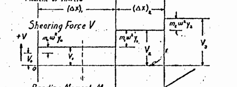
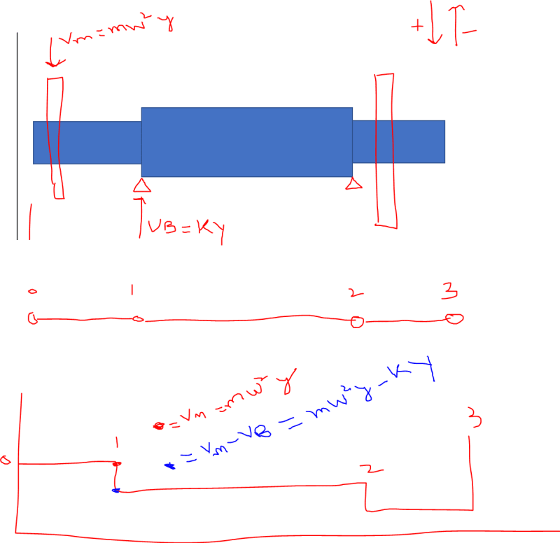
I just wanted to clarify one thing , shear force at bearings does indeed change , but logically the shear force at bearings would be as mentioned in the picture ,attached , where the shear due to bearing is upwards while the shear on the left of bearing would be purely due to inertia that is downwards , this means at bearing there is reduction of shear isnt it ? , please check the picture for reference . For some reason though the shear diagram in the paper adds mw^2y to V0 , Where Vo is the bearing reaction , its not subtracting it , I have attached that picture as well (black and white).

Your answer would be appreciated.


Shear1_wdmebz.png


Shear_islhlf.png
 
I wrote Vmiddle = Vleft - Kbrg*x ... but it should have been Vmiddle = Vleft - Kbrg*y since of course y is the vertical/lateral coordinate in our figures.

If y is positive that means the shaft is above its equilibrium position and the linearized bearing spring exerts a downward force on the shaft which acts in a direction to restore the shaft to equilibrium position. So shaft y positive means the bearing force applied to the shaft is negative. In my selected sign convention (which is not the only possible sign convention) while going from left to right, an upward force exerted upon shaft increases shaft shear V, while a downward force on the shaft decreases shaft shear, so my equation is consistent with my selected convention.

It's not clear to me what your figure is showing. A couple things to consider:
[ul]
[li]* The relevant force for shaft shear is force on the shaft (not the equal/opposite reaction force in the bearing)[/li]
[li]* If a point force is applied to the shaft (which is the way we're modeling it) then the shaft shear undergoes a step change from the left side of the node to the right side of the node. Your arrows are pointing at center of nodes so I'm not clear what that means. In my own terminology the node characteristics (and therefore the point forces) are captured in the point matrix which translates Sleft to Smiddle.[/li]
[/ul]

EDIT - I do see now your shear profile has a step change down at the location Vb. That step change down would be consistent with my own convention if the force on the shaft at that location was down. DELETED So if your upward arrow is intended to represents an upward reaction force on the bearing at that location, then the force on the shaft would be down at that location and that depicted step change would be consistent with my convention.DELETED

I apologize if I have told you things you already know, and I suspect I misunderstood your figure and your question. Feel free to rephrase your question and I'll try again.


@electricpete

Hi , thank you once again ,

I understand the shear in the shaft (Except at bearing points) is due to centrifugal loading which is active not reactive , at bearings though it is a combination of centrifugal force and bearing force isn't ?

Please refer to diagram attached with this email, the shaft is descretised as lumped mass at each station.


imagine the disk forces are pulling the shaft e.g at station 1, VM =mw^2y is downwards shown as red point (Vleft), the bearing force Vb= ky would be upwards won't it ? therefore the force represented by blue point is Vm-Vb also called the (Vright). y down is positive y up is negative in this case , the shaft depicted is at a state where the centrifigal forces are downwards.

would you not agree with it ?

see picture below:

Shear2_hilhiz.png


if you do why is the Vo in the black and white diagram shown below an addition of bearing force to the centrifugal force and not the subtraction, doesn't make sense to me.

Shear1_xznrwz.png


if you get time could you see why in the pdf paper is sent you ?


Thank you

AbdAlBasit
 
at bearings though it is a combination of centrifugal force and bearing force isn't ?
Yes, if you have a lumped mass at every node as you said below then you'll have a lumped mass at the same node as the bearing and the force applied to that node would be a combination of bearing force and centrifugal force.

imagine the disk forces are pulling the shaft e.g at station 1, VM =mw^2y is downwards shown as red point (Vleft), the bearing force Vb= ky would be upwards won't it ? therefore the force represented by blue point is Vm-Vb also called the (Vright). y down is positive y up is negative in this case , the shaft depicted is at a state where the centrifigal forces are downwards.
would you not agree with it ?
I'll assume Vm and Vb are positive quantities and their polarity is shown by the arrows.

The on the far left (to the left of the disk where Vm is applied), the shear is 0 (free boundary condition).

Between the location of the disk (where Vm is) and the bearing (where Vb is), the shear jumps to -Vm

To the right of the bearing since the bearing exerts downward force on the shaft, the shear jumps to -Vm + Vb.

That's similar to what you have except your polarity convention for shear reversed from mine. My convention is that as we go from left to right the shear increases where an upward force is applied.
if you do why is the Vo in the black and white diagram shown below an addition of bearing force to the centrifugal force and not the subtraction, doesn't make sense to me.
You're referring to figure 1 on page A143.
The equation above the figure says V1 = V0 + m0 w^2 y0 which seems to be consistent with my convention (positive/upward force causes increase in V as move left to right). Equation 19 supports the same conclusion (same convention).

I agree it's a strange figure. The curve of y isn't drawn so it's tough to know whether y at a given location is assumed + or -. I think we have to assume y0, y1 and y2 are all positive for the stepwise increase in V to make sense.

Based on the text above Figure 1, the bearing might be assumed at the left end position 0 (more later (*) ).

So let's initially assume bearing is at position 0. Since y0 is positive the bearing force would be negative and the change in shear would be negative. But that is not what is shown (he shows an increase of V0 at position 0). It's a contradiction.

A bearing at position 0 is not consistent with the figure since the polarity of the changes in shear associated with the bearing force and the centrifugal force should be in opposite directions (regardless of which convention is used). But he shows both in same direction, so it's a contradiction (which is what you were pointing out). It suggests to me that we have interpretted the bearing location wrong...

(*) I don't think he intends a bearing at position 0. He says "Assume that the following quantities are known at the left end of the system". That would be just setting the stage for the initial condition for integration without giving a lot of details. The comment "V=shearing force (due to bearing reaction)" was probably offhand and misleading. He is not attempting to characterize the whole rotor with this figure or comments (otherwise where is the other bearing). If the bearing he had in mind was at position 0 then I'm pretty sure he would have drawn a bearing at position 0 in the figure itself. But he didn't draw it there. So I'm pretty sure V0 is just the starting point, there is no jump in shear associated with a bearing at 0, he is not telling us anything about anything to the left of 0... other than that the shear reaches a value of V0 before we get to x=0. That could be stated more succintcly as V(x=0[sup]-[/sup]) = V0

That's my thought anyway, I could be mistaken. (Others are free to weigh in to see if they can make sense out of Figure 1)
 
@electricpete

Thanks so we are on the same page, with regards to Vo shearing force in his paper yes it cant be the shear at bearing.


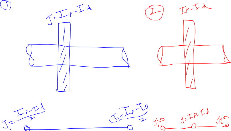
I had a simple quick question for you, to idealise the system into lumped mass system , where masses are concentrated at each node, for gyroscopic effects to be taken into account we also need to split the disc mass moment inertia among nearby nodes. How did you do that? My idea is using parallel axis theorm but its not helping me. for example. Imagine a disc between two shaft end points (the disc is not at the centre), you want to make a two node lumped mass idealisation, you can easily know the equivalent mass on each nodes by using principles of equilibrium . But to assign equivalent inertias to each node what would you do ? Can you explain with a plain example?

Thank you

Basit
 
Hi,

@electricpete, let me know when you get time.


Basit
 
I rely on my xfmatdisccussion3.pdf

For crticial speed calculation, J = Ip – Id
J = (1/2) rho L pi (R_outer[sup]4[/sup]-R_inner[sup]4[/sup])
where R_outer and R_inner are outer and inner radius of the disk.

So it represents the inertia of a disk which is distributed over a length L.

If the disk of length L spans between two nodes then each node gets half the value of J.

If the disk of length L has a node at each end and a node in the middle then we can view it as to disks of length L/2, each of which contributes half at each end. So the final result is that each of the outer nodes get J/4 and the center node gets J/4.

So in summary, J splits in a straightforward manner, just like you would split a distributed mass by putting half onto the node at each end. Arguably this is possible because (as discussed at bottom of page 3 of xfmatdisccussion3.pdf) the version of J that I'm using is the thin disk version which is proportional to L to the first power (just like mass of a disk is proportional to L to the first power). If you were using the long-disk version it is proportional to L^3 and it seems that could be tricky to split up especially in the case where a disk spans more than 2 nodes. But in all the cases I checked the thin disk version works fine to match results from other sources (even when the disk spans across several nodes).
 
@Electricpete,

so would the picture agree with what you are saying I only have these two cases for now. The only thing I don't understand from this is where is that half split coming from , is there any proof using parallel axis theorm or it is just an approximation?


Thank you

Basit
Inertia_obhie2.png
 
I intended to reply but forgot. Better late than never (?)...

I don't think parallel axis theorem would work. The axes of both halves are the same.

The split is analogous to splitting a continuous section mass M into M/2 at each adjacent node.

In the continuous case, the force or moment from accelerating the associated inertia is spread uniformly along the axis of the shaft.

In the discretized case, the approximate (*) same force or moment is split into two parts, separated axially by the distance between nodes.

(*) If there were something non-linear like a dependence on axial lenght squared, then that wouldn't work. But the thin-disk J formulas I provided are proportional to the axial length tot he first power (contrast to diameter which is not linear). And the forces or moment is directly proportional to that J. So all of that leads us to believe it will be a reasonable approximation which will become more exact as the separation distance decreases (finer discretization). I also didn't invent that approximation, it is used by many authors. If I recall some authors presented thumbbules for how fine discretization should be. Off the top of my head I think slicing any attached disk into pieces whose length is less than 20% of disk diameter and less than 50% of shaft diameter works pretty well to give reasonably accurate results. I don't have any proof or recall any authors presenting proof.
 
Modern formulas for statics and dynamics: A stress-and-strain approach BY PILKEY AND CHANG is a good source for transfer matrix methods. Walt Pilkey had a set of pregrams.

E. G. Pestel and F. A. Leckie, Matrix Methods in Elasto-Mechanics is great to understand the approach.


Regards,

Bill
 
Status
Not open for further replies.

Part and Inventory Search

Sponsor