Spring-mass-damper system subjected to impulse force - no vibrations

[BioMes]

Hello everyone!

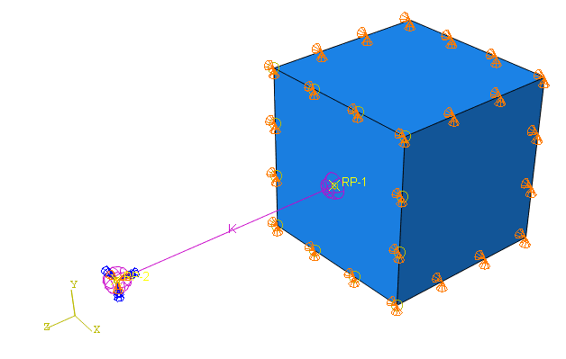
I'm working on a simple benchmark problem involving a spring-mass-damper system (for which I can get an analytical solution) modeled like this in Abaqus:

Currently, the damper is represented as modal damping with critical damping fraction for the natural frequency defined in the analysis step. The procedure is (transient) modal dynamics with a step time of 4 s and time increment of 0.1 s, utilizing a single mode shape from the preceding eigenfrequency extraction step. As you can see, the mass is simply a cube connected with a spring via a rigid body constraint. The spring is fixed at the other end.

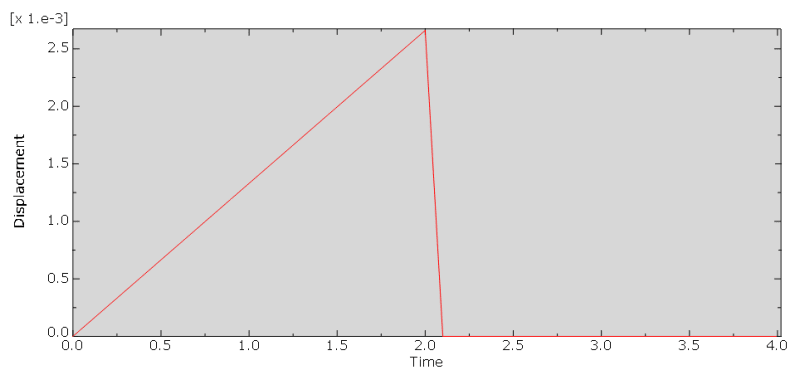
A tensile load is applied to the opposite side of the cube and the following amplitude is used for it:

The problem is that I don't get any vibrations in results. Just a response (displacement of one of the nodes of the cube) equivalent to the applied amplitude and with the final displacement close to 0 (according to the analytical solution it shouldn't be zero for t=4 s):

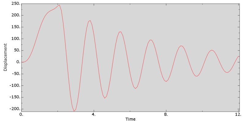
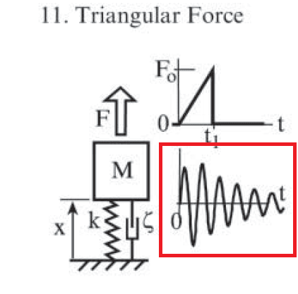
I would expect a response like this (from the Blevins' book):

Am I missing something here?

 

[GregLocock]

That rather depends on the specific values of k m and c in your model.

Cheers

Greg Locock


New here? Try reading these, they might help FAQ731-376

http://eng-tips.com/market.cfm?

 

[BioMes]

Thank you for the reply. I made up those values for the benchmark problem. Here they are:
- the box is 60x60x60 mm and has a density of 8000 kg/m^3 meaning that the mass is 1.728 kg
- the spring stiffness is 75398 N/mm
- the damping coefficient equals 0.02

Is there a way to calculate the values required to obtain the expected vibrational response? I don't understand why the displacement drops to almost zero. The damping coefficient doesn't seem so large.

 

[Denial]

Despite the distraction of the large cube, you appear to have what is in effect a single degree of freedom model. Thanks to Greg's query, we now know that the sprung mass is 1.748[ ]kg and the spring stiffness is 75398000[ ]N/m. So your natural frequency is about 1051[ ]cycles per second.[ ] Your structure is seeing your applied load profile as a (very) gradually varying load rather than a dynamic load, so the "shape" of your displacement versus time output is very close to the "shape" of your load versus time input.

It seems that this is not what you expected.[ ] You must have set your model up wrongly somehow.[ ] Inconsistent units??

[sub][ ]—————————————————————————————————[/sub]
[sup]Engineering mathematician / analyst.[ ] See my profile for more details.[/sup]

 

[rb1957]

since yo can solve this by hand, what is your hand solution to this problem ? is it very heavily damped ??

maybe interrogate the output displacement ? maybe it is not as linear as it looks ??

"Hoffen wir mal, dass alles gut geht !"
General Paulus, Nov 1942, outside Stalingrad after the launch of Operation Uranus.

 

[BioMes]

The analytical solution for the values listed above is x(4 s)=4.9497e-5 mm which is nowhere near the numerical result but it's likely because of that issue with unexpected response (no vibrations).

When I decreased the spring stiffness by several orders of magnitude (to 0.75398 N/mm) and increased the mass (to 54.286 kg), I got a much better response:

Now the analytical solution is 106.76 mm so way closer to the simulation result (118.923 mm) but still with some visible difference. However, those new values seem to be unrealistic. The problem is that I have absolutely no sense when it comes to selecting inputs for such an abstract benchmark example. I selected those initial values based on the fact that I wanted to model the mass as a cube of a reasonable size (60x60x60 mm) and the spring as a rod of 140 mm length and 8 mm diameter also made of steel with E=210 GPa (hence the calculated stiffness).

@Denial is likely also right that the impulse could be shorter to trigger the dynamic response (so maybe something like ramp from 0 to maximum force in a fraction of a second instead of 2 seconds). I don't want to enter high-speed dynamics here but the current amplitude can be more quasi-static than dynamic. I have to play with those values.

 

[karachun]

Hello, BioMes. I have a couple of questions on your setup.
1) Why not use mass element instead of solid cube so you can directly input mass and have real 1DOF system. I don`t know how to create mass in Abaqus but I don`t think that it is difficult.
2) In first setup your time increment is too coarse. According to mass and stiffness system natural frequency would be f=(k/m)^0.5/2/pi = (75398000/1.748)^0.5/2/pi = 1045 Hz, oscillation period would be 1/1045 ~ 1e-3 s. With time increment of 0.1 s you got 100 unresolved oscillations between two calculated time points! You can not chose timestep randomly. You should perform timestep convergence to ensure that your solution does not depend from timestep size. You can start with time increment size of something like 1/10 of natural oscillation period. It would be 1/1045/10 ~ 1e-4 s. Then you should make 2-3 additional analysis with time increment gradually reduced by factor of 1.5-2 until you notice that result (displacement in your case) almost stop changing and further reduction of timestep don`t change results.

Note that if your timestep is greater than half of 1DOF period than your results are wrong due to Nyquist–Shannon sampling theorem.

https://en.wikipedia.org/wiki/Nyquist–Shannon_sampling_theorem

I don't want to enter high-speed dynamics here but the current amplitude can be more quasi-static than dynamic. I have to play with those values.

You have some wrong understanding of how linear dynamics works. You do not need to use some nonlinear high speed dynamics. You just reduce timestep size but your system is still linear.

Therefore first calculate your system natural frequency and period (using hand calculation and FEA) and than select appropriate timestep size. All dynamics starts from natural frequency analysis, don`t neglect it.

And for loading I suppose that loading time t1 should be less than one period of oscillation.

 

[BioMes]

@karachun

Thank you for your valuable tips.

In fact, I'm working on 2 test models and one of them indeed uses point mass element. The other one (with the mass modeled as a cube) is meant to be more versatile so that it can be used in other software, not supporting mass elements. That's also why I modeled the spring as a solid rod and calculated its equivalent stiffness initially.

You are right about the time increment, I forgot about the necessity of its adjustment. However, it's not the cause of the unexpected response here since it doesn't really change my results - for the first case the resulting displacement still directly reflects the excitation and is zero after the impulse ends when I use 1e-4 as the time increment. For the second case, the result is also the same (good but not perfectly agreeing with the analytical calculations) when I change the time increment from 0.1 to 0.01 (the natural frequency is 0.59 Hz in this case).

I guess that I just have to play with k and m values and maybe I will get a bit closer to the analytical result. I will also try with a shorter impulse.

 

[karachun]

I guess that I just have to play with k and m values and maybe I will get a bit closer to the analytical result.

In this case you can just write numbers you want and not bothering with analysis.

To get accurate results you first need to ensure that your input is correct. Here I write input and some pitfalls that may occur (maybe other users can add to this list).
1) Mass and stiffness.
2) Damping. What type of damping? Part of critical damping, viscoelastic damping of Q-factor? There are many methods to define damping you should clarify that you use same method as defined in book.
3) Load. What are book recommendations of load application method? Is it rapid (t1 less than one period of oscillation(T)) of quasi static (t1 is many times greater that T). For quasi static method load time is irrelevant but is loading is rapid than different loading time give different results.
4) Timestep - checked, timestep must be small enough.
5) Analytical results. How you calculate them, it is possible that you made some mistakes? It will be good if you provide formulas from your book and share your calculations for those who don`t have this book. Personally i even don`t know this author.

If you clarify every item from this list than someone can recreate your problem in Abaqus and post input file. i am not an Abaqus user but i can make this problem in Nastran and than can export it into Abaqus format if I get reasonable results. But without good input data it is a black box because now you have posted two or three different sets of initial data and results simultaneously.

 

[GregLocock]

ChatGPT can write a perfectly good script to analyse SDOF linear systems, in about 20 lines.

Cheers

Greg Locock


New here? Try reading these, they might help FAQ731-376

http://eng-tips.com/market.cfm?

 

[IceBreakerSours]

ChatGPT is already baked into Mathematica and collimator.ai.

*********************************************************
Are you new to this forum? If so, please read these FAQs:

http://www.eng-tips.com/faqs.cfm?fid=376

http://www.eng-tips.com/faqs.cfm?fid=1083

 

[GregLocock]

Here's the calulations

https://engcourses-uofa.ca/books/vi...nse-of-spring-mass-system-to-a-ramp-function/

But in your case the ramp is very slow compared with the resonant frequency of the system, so you'll just get the spring stiffness.

Cheers

Greg Locock


New here? Try reading these, they might help FAQ731-376

http://eng-tips.com/market.cfm?

 

[BioMes]

I was testing different k and m values. I got not so bad results for the last data set shared here (with f_n = 0.59 Hz): 138.35 mm from the simulation vs 106.76 mm from the analytical calculations. But for other values of k I don't get any agreement. Here's the current information:

1. Input:
- mass: 54.286 kg
- stiffness: 7.5398 N/mm
- natural frequency: 1.8757 Hz

2. Damping:
ξ = 0.02
The book defines it as "dimensionless damping factor also called the damping ratio and fraction of critical damping". I define it as "modal damping" and specify the fraction of critical damping so it should be correct.

3. Load:
F= 200 N
The book doesn't provide any recommendations, it only describes the load as "triangular force". It's just one of the cases from a table (like in Roark's).

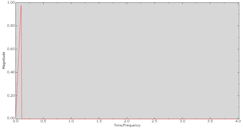
I changed the amplitude to make the impulse shorter. Currently the amplitude is:
t A
0 0
0.1 1
0.11 0
4 0

4. Timestep:
t_i = 0.01 s since (1/1.8757)/10 = 0.0533 s

5. Analytical results:

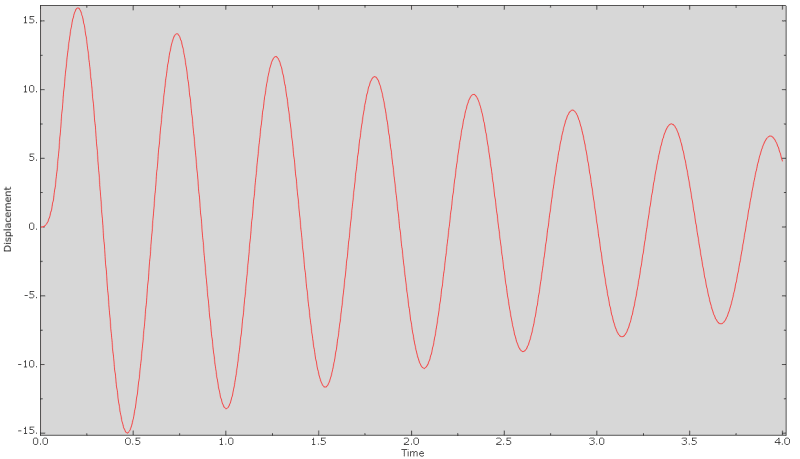
Currently, there's no agreement. For t=4 s I get 4.77 mm from the simulation and 16.94 mm from the analytical calculations. Here's the response from the analysis:

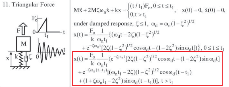
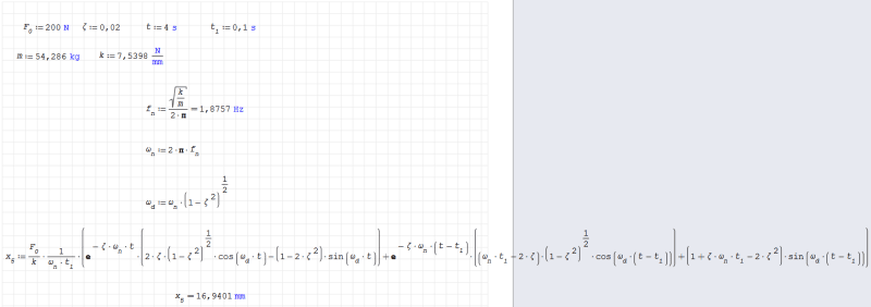
The formula from the book:

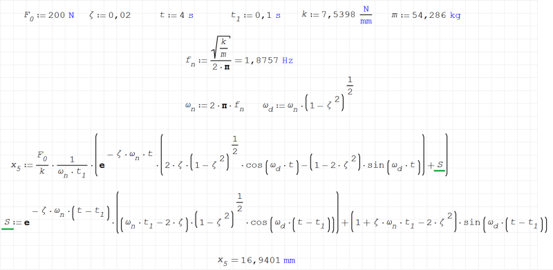
And my calculations (should be correct since I'm using SMath):

Any ideas what can be wrong?

 

[GregLocock]

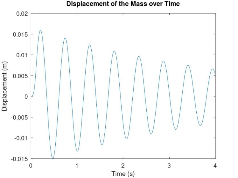
You've now shortened the ramp, so it is more like a pulse excitation. At t=0.1 the velocity should be 200/2/54*.1 m/s, so the simple harmonic motion amplitude ie the first peak should be .2 m/s/12 rad/s=16mm ish, so check your analytical for that

Cheers

Greg Locock


New here? Try reading these, they might help FAQ731-376

http://eng-tips.com/market.cfm?

 

[GregLocock]

%Greg Locock/ChatGPT
%2023 jul 4
%To do
%
%
%Dependency

clear all
close all
% Parameters
m = 54.286;    % Mass (kg)
k = 7539.8;    % Spring constant (N/m)
cv = 0.02*2*m*sqrt(k/m);    % Damping coefficient
F = 200;       % Magnitude of applied force (N)

% Time settings
dt = 0.01;     % Time interval (s)
totalTime = 4; % Total simulation time (s)
numSteps = totalTime / dt;

% Initial conditions
x0 = 0;        % Initial displacement
v0 = 0;        % Initial velocity

% Preallocate arrays for storing results
t = zeros(numSteps, 1);
x = zeros(numSteps, 1);
v = zeros(numSteps, 1);

% Runge-Kutta integration
for i = 1:numSteps
    % Current time
    t(i) = (i - 1) * dt;

    % Determine if the force is applied during the interval 0 to 0.1 seconds
    if t(i) >= 0 && t(i) <= 0.1
        F_applied = F*t(i)/.1
    else
        F_applied = 0;
    end

    % Calculate acceleration
    xdd = (F_applied - eta * v(i) - k * x(i)) / m;

    % Update velocity and displacement using Runge-Kutta method
    k1 = dt * v(i);
    l1 = dt * xdd;
    k2 = dt * (v(i) + 0.5 * l1);
    l2 = dt * ((F_applied - cv * (v(i) + 0.5 * l1) - k * (x(i) + 0.5 * k1)) / m);
    k3 = dt * (v(i) + 0.5 * l2);
    l3 = dt * ((F_applied - cv * (v(i) + 0.5 * l2) - k * (x(i) + 0.5 * k2)) / m);
    k4 = dt * (v(i) + l3);
    l4 = dt * ((F_applied - cv * (v(i) + l3) - k * (x(i) + k3)) / m);

    x(i+1) = x(i) + (k1 + 2*k2 + 2*k3 + k4) / 6;
    v(i+1) = v(i) + (l1 + 2*l2 + 2*l3 + l4) / 6;
end

% Plotting

plot(t, x(1:400))
xlabel('Time (s)')
ylabel('Displacement (m)')
title('Displacement of the Mass over Time')

which agrees with your plot pretty well. Your unreadable smath is probably wrong

Cheers

Greg Locock


New here? Try reading these, they might help FAQ731-376

http://eng-tips.com/market.cfm?

 

[BioMes]

Thank you very much for this numerical solution. Did you have to make many corrections to what ChatGPT generated?

I would like to correct my analytical solution anyway. You are right that it was too hard to read. This one should be much better:

I checked the formula a few times but maybe I missed some mistake that you will notice. Or the equation in the book is incorrect... I couldn't get agreement with equations for harmonic loading of beams from this book as well.

 

[GregLocock]

A few edits that were quicker to do directly, the RK section is unchanged. It got the eta calculation wrong, just ignored the conversion to cv.

Cheers

Greg Locock


New here? Try reading these, they might help FAQ731-376

http://eng-tips.com/market.cfm?

 

[BioMes]

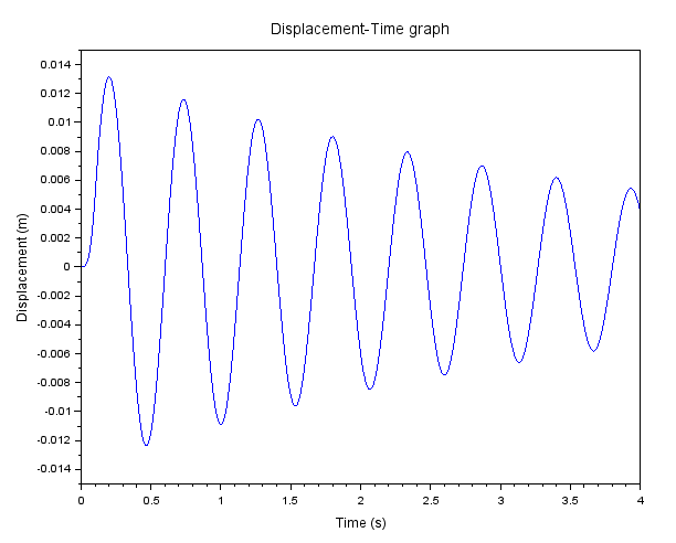
I don't have access to Matlab so I asked ChatGPT to generate a similar code for SciLab. Here's what I got:

// Constants
m = 54.286;     // mass (kg)
k = 7539.8;     // spring stiffness (N/m)
cv = 0.02 * 2 * m * sqrt(k / m);  // damping coefficient
F = 200;        // force (N)
dt = 0.01;      // time interval (s)
total_time = 4; // total time (s)

// Number of time steps
N = total_time / dt;

// Initializing variables
u = zeros(N+1, 1); // displacement
v = zeros(N+1, 1); // velocity

// Initial conditions
u(1) = 0;
v(1) = 0;

// Triangular impulse force function
function F_i = force(t)
    if (t >= 0) & (t < 0.1)
        F_i = (200 / 0.1) * t;
    else
        F_i = 0;
    end
endfunction

// Runge-Kutta integration
for i = 1:N
    t = (i - 1) * dt;
    F_i = force(t);
    
    k1u = v(i) * dt;
    k1v = (F_i - k * u(i) - cv * v(i)) / m * dt;
    
    k2u = (v(i) + k1v/2) * dt;
    k2v = (F_i - k * (u(i) + k1u/2) - cv * (v(i) + k1v/2)) / m * dt;
    
    k3u = (v(i) + k2v/2) * dt;
    k3v = (F_i - k * (u(i) + k2u/2) - cv * (v(i) + k2v/2)) / m * dt;
    
    k4u = (v(i) + k3v) * dt;
    k4v = (F_i - k * (u(i) + k3u) - cv * (v(i) + k3v)) / m * dt;
    
    u(i+1) = u(i) + (k1u + 2*k2u + 2*k3u + k4u) / 6;
    v(i+1) = v(i) + (k1v + 2*k2v + 2*k3v + k4v) / 6;
end

// Plotting the displacement-time graph
t = linspace(0, total_time, N+1);
plot(t, u)
xlabel('Time (s)')
ylabel('Displacement (m)')
title('Displacement-Time graph')

The resulting plot is almost the same but with some difference in values:

I wonder what caused it.

 

[GregLocock]

beginner error t<=0.1 (the same mistake I made in my first ever Fortran program)

Cheers

Greg Locock


New here? Try reading these, they might help FAQ731-376

http://eng-tips.com/market.cfm?

 

[BioMes]

Right, now it looks like your plot and the value for t = 4 s is 4.8 mm (previously it was 4.68 mm) while the simulation result is 4.77 mm. Close enough.

I still wonder if this analytical solution utilizing the formula from the Blevin's book ("Formulas for Dynamics, Acoustics and Vibration") can be fixed and provide correct results. I've got no idea what can be wrong with it.