VBA CODE - Tracking work hours

[Kenja824]

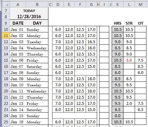
I am looking to make a module(s) that will help me keep track of hours worked each week. The pic below is the basic idea of my format. Specifically, what I am looking for is what will come up in columns L and M in the pic.

*Each w

http://www.eng-tips.com/threadminder.cfm?pid=766eek

starts on Monday and ends on Sunday.

In column L, it will display the STRAIGHT time hours for each day.

In column M, it will display only the OVERTIME hours for each day. (anything over 40 hours for the week)

In Column K, I already have the formula .... =SUM(IF(E10>D10,E10-D10,"0"))+(IF(G10>F10,G10-F10,"0"))-I10 .... The code for L & M can recalculate the punch in and punch out times, or it can be derived from the totals of column K, whatever is easiest, I will work with.

NOTE: If you can do this with simple formulas that can be copied down the two columns, that would work for me too. I just figured this might be easier to write VBA code for if you know it. I have been struggling to learn it for a while and my understanding of VB and VBA code is coming very slowly. Veeeeerrryyyyy sllooooo

http://wwwwlllyyyyy.....

lol It may be hindering me that I am trying to learn both at the same time. Not sure.

if this is not too difficult and you can help me with this, it will be greatly appreciated, as not only will it get me what I need, but it will give me more code to read and understand and learn from. )

Please ignore the fact one number is red.

Hope everyone had a wonderful Christmas and has a great New Year.

 

[onlyadrafter]

Hello,

If you can add two columns (to make this easier) then you can do the following:

In N10 enter this formula:

=WEEKNUM(C10,2)

In O10 enter this formula:

=SUMIF($N$10:N10,WEEKNUM(C10,2),$K$10:K10)

In L10 enter this formula:

=IF(O10>40,K10-M10,K10)

In M10 enter this formula:

=IF(AND(N9>40,O10>40),K10,IF(O10>40,O10-40,0))

copy these down as far as required.

There is probably a simpler solution, but not the best as time calculations. However, this does give the same results as your post.

You could combine the 'extra' formulas into cols L & M.


----------------------------------
Hope this helps.
----------------------------------

been away for quite a while
but am now back

 

[Kenja824]

Hey Onlyadrafter

Thanks for the help. At first these did not work, but I realized you were naming cell C10 in a couple of the formulas and that cell is empty at this time. I assumed you meant A10 to get the day of the week? This seemed to work at first but when I dragged it down, I the STR column (L) would continue to give amounts after it totaled 40 hours for the week, only the amounts returned were a negative of the cell one up in the L column.

I was able to fix this by making the formula in "L10" to be....
=IF(IF(O10>40,K10-M10,K10)<0,"",IF(O10>40,K10-M10,K10))
So that if it became a negative number, it would return as a blank cell.

For M10, I changed the "0" return to "" as well to get my preferred results....
=IF(AND(N9>40,O10>40),K10,IF(O10>40,O10-40,""))

I get the feeling there is an easier and cleaner way. Most likely with a VBA code, but this gets the job done. If in playing with it I find a cleaner way, I will post it.

Thanks for the help.

 

[onlyadrafter]

Hello,

You are correct, I did mean Cell A10, not C10.

Have attached the file I created. I also copied the data down to try and replicate what you found, but it still appears to give correct results.

----------------------------------
Hope this helps.
----------------------------------

been away for quite a while
but am now back

 

[Kenja824]

Interesting. So I found why I was getting negative numbers. The code in your post above for M10 ... =IF(AND(N9>40,O10>40),K10,IF(O10>40,O10-40,0)) .... has an N9. In the file you loaded for me, the cells below that all have O10, O11 instead of N10 and N11. So when I copied it and pasted it with the N and dragged it down, it gave me a negative number.

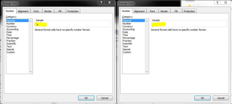
The interesting thing is that I found why I need to use the "" to get a blank cell and you dont. I showed the formatting for the same cell for each of our files in the pic below. I just have no idea why its like this and how to fix it. lol

 

[onlyadrafter]

Hello,

Oops. Just spotted that. The formula in M10 should be:

=IF(AND(O9>40,O10>40),K10,IF(O10>40,O10-40,0))

copy this down as far as required.

The reason I have blank cells, is that in the FILE, OPTIONS, ADVANCED. Display Options for this Worksheet, I have unchecked the display zeros.

Does it work as expected?

----------------------------------
Hope this helps.
----------------------------------

been away for quite a while
but am now back

 

[Kenja824]

Wow, I even looked in the options for that, expecting it had to be there and couldnt find it. Im guessing it was one of my brighter moments and I didnt realize at the time that the advanced area can be scrolled down. lol

Yes, the formulas do work how I was hoping. If anyone ever has time to write the code for it I would still like to have that for my learning purposes, but for now this does work. Thanks Onlyadrafter. You might need to change your handle to Morethanadrafter soon. lol

 

[Kenja824]

Also, just to add to this, I was able to use some of my old formula and make it so we dont need the formula in column N anymore. The formula in O10 is now .... =IF(WEEKDAY(A10)=2,K10,SUM(K10+O9))

 

[onlyadrafter]

Hello,

Does this work as expected?

Column N needs to be empty though.

Sub TRACK_HOURS()
    Application.ScreenUpdating = False
'PUT WEEK NUMBER IN COL N
    For MY_ROWS = 10 To Range("A" & Rows.Count).End(xlUp).Row
        Range("N" & MY_ROWS).Formula = "=weeknum(A" & MY_ROWS & ",2)"
    Next MY_ROWS
'CALCULATE HOURS
    MY_CURRENT_WEEK = Range("N10").Value
    For MY_ROWS = 10 To Range("A" & Rows.Count).End(xlUp).Row
        MY_TOTAL = MY_TOTAL + Range("K" & MY_ROWS).Value
        If Range("N" & MY_ROWS + 1).Value <> Range("N" & MY_ROWS).Value Then
            If MY_TOTAL <= 40 Then
                Range("L" & MY_ROWS).Value = Range("K" & MY_ROWS).Value
                MY_TOTAL = 0
            Else
                If MY_TOTAL <= 40 Then
                    Range("L" & MY_ROWS).Value = Range("K" & MY_ROWS).Value
                Else
                    Range("M" & MY_ROWS).Value = Range("K" & MY_ROWS).Value
                    MY_TOTAL = 0
                End If
            End If
        Else
            If MY_TOTAL <= 40 Then
                Range("L" & MY_ROWS).Value = Range("K" & MY_ROWS).Value
            Else
                If Range("M" & MY_ROWS - 1).Value > 0 Then
                    Range("M" & MY_ROWS).Value = Range("K" & MY_ROWS).Value
                Else
                    Range("M" & MY_ROWS).Value = MY_TOTAL - 40 'Range("K" & MY_ROWS).Value
                    Range("L" & MY_ROWS).Value = 40 - (MY_TOTAL - Range("K" & MY_ROWS).Value)
                End If
                If Range("N" & MY_ROWS + 1).Value <> Range("N" & MY_ROWS).Value Then
                    MY_TOTAL = 0
                End If
            End If
        End If
    Next MY_ROWS
        Columns("N:N").ClearContents
        Application.ScreenUpdating = True
End Sub

I'm sure this code can be shortened, but it's been a really long day.

----------------------------------
Hope this helps.
----------------------------------

been away for quite a while
but am now back

 

[Kenja824]

Ok, here is where I have to be most honest..... I have no idea if this works right. lol This is how green I am with VBA Code. I was thinking more in the lines of modules I would add and then click on the cell, hit = and find the new function. lol The more I think on it, I can see where that would need multiple functions and such. I sat there trying to find this one when I hit the = and finally realized it is ran as a macro.

So I saved where I was and hit run and it flickered but I have no idea what it did if it did anything. The problem is that I have been messing with my sheet for a bit and added columns and such. The only way I will know if it works is if I go through the code and see what exactly it does and change my excel form to be set in a way that I will know if it actually did something or not. And I leave in a few and will be off until after the New Year.

Man I wish I had excel at home to mess with this stuff. lol

However, the important thing is, I will get to go through this when I can and if nothing else will learn from the code and that is what I wanted more than anything.

I really appreciate everything Onlyadrafter. The formula help got me on track for what I wanted to do and I will learn what I can from the code when I get back to it. Hope you have an awesome New Year and a better whole Year. )

 

[SkipVought]

Two comments.

1)

http://www.Tek-Tips.com

(you should see this link just under the URL bar, alon with Eng-Tips and Engineering.com) is where you can get lots of coding & spreadsheet tips.

2) you really ought to upload a sample workbook or at least post a useable copy 'n' past sample. If you won't take the time to do that, many of us won't waste the time transcribing your data picture into a useable table.


Skip,
[sub]
Just traded in my OLD subtlety...
for a NUance![/sub]

 

[SkipVought]

BTW, a spreadsheet solution...
[pre]
Date Day WkNo HRS ST OT
Jan 02 Mon 2 10 10 0
Jan 03 Tue 2 8 18 0
Jan 04 Wed 2 12 30 0
Jan 05 Thu 2 8 38 0
Jan 06 Fri 2 8 40 6
Jan 07 Sat 2 10 40 16
Jan 08 Sun 2 10 40 26
Jan 09 Mon 3 8 8 0
Jan 10 Tue 3 8 16 0
Jan 11 Wed 3 8 24 0
Jan 12 Thu 3 9 33 0
Jan 13 Fri 3 9 40 2
Jan 14 Sat 3 9 40 11
[/pre]

ST E4: =IF(SUMPRODUCT(($C$4:C4=C4)*($D$44))<=40,SUMPRODUCT(($C$4:C4=C4)*($D$44)),40)
OT F4: =SUMPRODUCT(($C$4:C4=C4)*($D$44))-E4

Skip,
[sub]
Just traded in my OLD subtlety...
for a NUance![/sub]

 

[SkipVought]

What would be even easier is to just track your hours by day using Named Ranges...
[pre]
Date Day WkNo HRS
Jan 02 Mon 2 8
Jan 03 Tue 2 8
Jan 04 Wed 2 8
Jan 05 Thu 2 8
Jan 06 Fri 2 8
Jan 07 Sat 2 0
Jan 08 Sun 2 0
Jan 09 Mon 3 8
Jan 10 Tue 3 8
Jan 11 Wed 3 8
Jan 12 Thu 3 9
Jan 13 Fri 3 9
Jan 14 Sat 3 9
Jan 15 Sun 3 9
Jan 16 Mon 4 10
Jan 17 Tue 4 10
Jan 18 Wed 4 12
Jan 19 Thu 4 8
Jan 20 Fri 4 10
Jan 21 Sat 4 10
Jan 22 Sun 4 8
Jan 23 Mon 5 8
Jan 24 Tue 5 12
Jan 25 Wed 5 8
Jan 26 Thu 5 8
Jan 27 Fri 5 8
Jan 28 Sat 5 12
Jan 29 Sun 5 10
Jan 30 Mon 6 9
Jan 31 Tue 6 8
Feb 01 Wed 6 8
Feb 02 Thu 6 12
Feb 03 Fri 6 10
Feb 04 Sat 6 10
[/pre]

Then just have a summary table like this using the Named Ranges in the table above...
[pre]
Week Of HRS ST OT
1/2/2017 40 40 0
1/9/2017 60 40 20
1/16/2017 68 40 28
1/23/2017 66 40 26
1/30/2017 57 40 17
[/pre]
...where
[tt]
HRS J4: =SUMPRODUCT((WkNo=WEEKNUM($I4,2))*(HRS))
ST K4: =IF(J4>40,40,J4)
OT L4: =J4-K4
[/tt]


Skip,
[sub]
Just traded in my OLD subtlety...
for a NUance![/sub]