Excel "VLOOKUP" to return a table of values 9

[MegaStructures]

Hello:

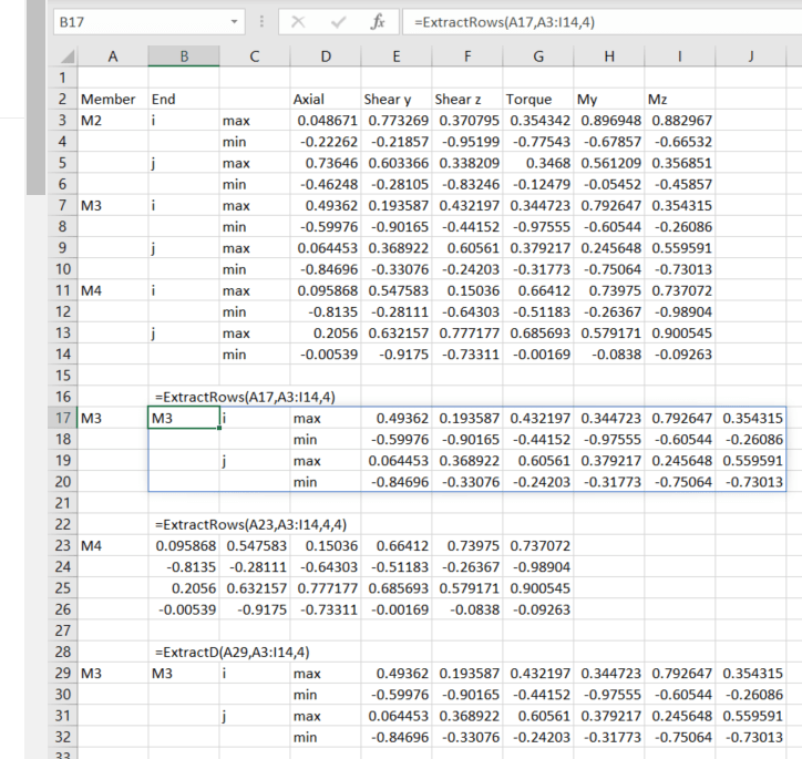
I have a situation where I have a native list coming out of a structural analysis program that comes with one identifier for a block of values 8 columns wide and 4 rows tall. I would like to find a way to call the entire table from another sheet by looking for the single identifier. Example of the information is below.

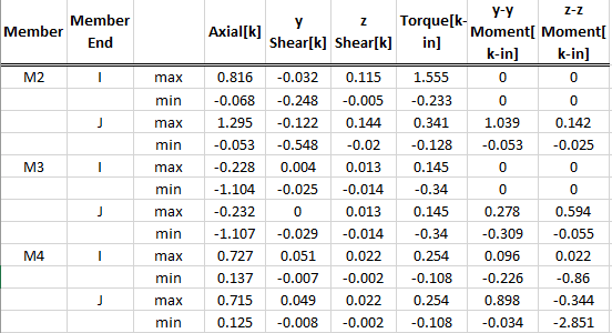
Is there a way to do this with a native excel function? Is there a relatively easy way to do this with VBA or Python?

“Any idiot can build a bridge that stands, but it takes an engineer to build a bridge that barely stands.”

 

[Agent666]

Filter function possibly? Base it on another helper column that you populate with the member reference?

 

[sticksandtriangles]

Python can definitely handle this, I'm sure VBA can as well, but I am not as versed in VBA.

S&T

 

[MegaStructures]

I've never used Python, so I assume the solution isn't easy enough to explain to a new beginner?

“Any idiot can build a bridge that stands, but it takes an engineer to build a bridge that barely stands.”

 

[SkipVought]

Hi,

Is this "table" for visual only or for the purpose of calculations in Excel? I suspect visual only.

If thats the case, you can use the Camera feature in addition to Naming the table range.

Maybe I misread your requirement. Where is the Identifier value with respect to other Identifiers??

I also see more columns than 8 and more rows than 4.

To reference this table EVERY row needs date. The implied value must be present in the table.

Skip,

_{Just traded in my OLD subtlety...
for a NUance!}

 

[MegaStructures]

The table is for calculations inside of excel. I basically want to do exactly what VLOOKUP does, but instead of returning a single cell it returns a 8x4 "table" of cells

“Any idiot can build a bridge that stands, but it takes an engineer to build a bridge that barely stands.”

 

[sticksandtriangles]

Sorry, I should have followed up with a little more direction.

In Python, dictionaries are the excel version of the vlookup function, denoted by these characters "{}". You feed a dictionary a key and value.

See below for an example:

row = [1,2,3,4,5,6]

data = []
data_1 = []
#make dummy data
for i in range(len(row)) :
    temp = []
    temp_1 = []
    for number in row :
        temp.append(number*i)
        temp_1.append(number*i/2)
    data.append(temp)
    data_1.append(temp_1)
    
    
print(data)
print(data_1)


key = 'M2'
value = data

key_1 = 'M3'
value_1 = data_1
#make dictionary
z = {key: value, key_1: data_1}


#pull values from dictionary
x = z["M3"]

print(x)

In this example, x is now equal to the "value" keyed to "M3"

x
Out[6]: 
[[0.0, 0.0, 0.0, 0.0, 0.0, 0.0],
 [0.5, 1.0, 1.5, 2.0, 2.5, 3.0],
 [1.0, 2.0, 3.0, 4.0, 5.0, 6.0],
 [1.5, 3.0, 4.5, 6.0, 7.5, 9.0],
 [2.0, 4.0, 6.0, 8.0, 10.0, 12.0],
 [2.5, 5.0, 7.5, 10.0, 12.5, 15.0]]

You can get even fancier with nested dictionaries where you could theoritically organize your data a little more.
something like: z['M3'][Axial]
this could then call just the axial results for 'M3', but the example above should hopefully give you enough to get going if you wanted to explore python

S&T

 

[SkipVought]

VLOOKUP will not work. You could use the OFFSET() function which returns a table array where...
Arg1 references the top-left of the entire table
Arg2 is the row offset of the Identifier
Arg3 is the column offset of the Identifier
Arg4 is the number of rows associated with the Identifier
Arg5 is the number of columns associated with the Identifier

Then use VLOOKUP or INDEX & MATCH on the OFFSET range.

BTW, an actual COPY n PASTE table would be helpful if you actually want to encourage a solution.

Skip,

_{Just traded in my OLD subtlety...
for a NUance!}

 

[MegaStructures]

SkipVought That seems like it could work beautifully if I could nest VLOOKUP in the reference argument

“Any idiot can build a bridge that stands, but it takes an engineer to build a bridge that barely stands.”

 

[MegaStructures]

SkipVought that worked perfectly. If I could give you two stars I would. Thank you.

sticksandtriangles, thank you for the effort you put into your explanation. I'm sure your solution works rather well too, I'm just a bit too slow to use it just yet . One day soon!

“Any idiot can build a bridge that stands, but it takes an engineer to build a bridge that barely stands.”

 

[SkipVought]

Sorry, I messed up my initial post.
It might be something like this...
[tt]
=OFFSET
(
IdentifierRng
,MATCH(SelectedIdentifier,IdentifierRng,0)-1
,1
,12
,9
)
[/tt]
...IF each block has 12 rows and 9 columns as your example has.


Skip,

_{Just traded in my OLD subtlety...
for a NUance!}

 

[SkipVought]

Here's my solution.

The source table is a Structured Table named tDATA in the Data tab.

The dashboard is in Sheet2
[pre]
2 1 4 5 6 7 8 9
SelectedIdentifier SelectedMember SelectedMemEnd SelectedMM Axial[k] y Shear[k] z Shear[k] Torque [k-in] y-y Moment [k-in] z-z Moment [k-in]
[highlight #FCE94F]A1 B J Max [/highlight] 0.55279 0.2027661 0.4646301 0.27592941 0.129484892 0.805786672
[/pre]

SelectedIdentifier is user entry in yellow
SelectedMember is user entry in yellow
SelectedMemEnd Is either 0 or 2 depending on I or J in the yellow user entry
SelectedMM Is either 0 or 1 depending on Min or Max in yellow user entry
These last 2 values add to the row offset for the Index function.

Formula in E3 calculates the correct parameter based on the selections.
[tt]
E3: =INDEX(OFFSET(tDATA[Identifier],MATCH(SelectedIdentifier,tDATA[Identifier],0)-1,1,12,9),
MATCH(SelectedMember,OFFSET(tDATA[Identifier],
MATCH(SelectedIdentifier,tDATA[Identifier],0)-1,1,12,1),0)+SelectedMemEnd+SelectedMM,E1)
[/tt]
The values in row 1 above the Data table headings are column offsets for the INDEX function.

Skip,

_{Just traded in my OLD subtlety...
for a NUance!}

 

[SkipVought]

You could also make a helper lookup column, concatenating the values Identifier, Member, Member End & MinMax. This assumes each row has these values. In my world they do.

I almost exclusively use Index & Match. I don't worry about having the lookup column first. It can be anywhere. If I were to make a lookup column, I'd put it to the right of the existing table. I'd make the INDEX range, just the columns of return data.

It's also possible to use the SUMPRODUCT() function IF and only if each row contains lookup values, which a true table ALWAYS does.
[tt]
=SUMPRODUCT(
(tDATA[Identifier]=SelectedIdentifier)*
(tDATA[Member]=SelectedMember)*
(tDATA[Member End]=SelectedMemEnd)*
(tDATA[MM]=SelectedMM)*
(tDATA[Axial'[k']])
)
[/tt]

Since your table seems to have fixed block sizes, it greatly simplifies specific row lookups where it seems you don't have lookup vaues in each row.

Skip,

_{Just traded in my OLD subtlety...
for a NUance!}

 

[Agent666]

Check attached for example of how to use filter function with a helper column to populate the member reference for each row.

Change the dropdown in cell K3 to choose desired member reference.

FILTER EXAMPLE.xlsx

EDIT - realise I left out the min/max in raw data. But you get the idea hopefully!

 

[IDS]

If this is going to be extensively used, a VBA UDF is worth looking into. The screenshot below shows two alternatives:
ExtractRows(RowID, DataRange, Rows = 1, FirstCol = 1, Cols = 0)
or ExtractD(same input)

The two functions are the same except ExtractRows steps through the first column until it finds the RowID, and ExtractD creates a dictionary of RowIDs and the associated row number.

They both return an array of the number of rows specified in Rows (default 1), starting at FirstCol (default 1) up to the end, or the number of columns specified in Cols. Note that the Rows value should be equal to the spacing of the Member ID text.

With the code as is I doubt there is any advantage in using a dictionary, in fact quite likely it is slower, but it would be easy to extend the code to read a list of Member IDs (not necessarily sequential), and return a single table for all of them. In that case the dictionary would definitely be quicker.

The functions use the new Excel dynamic array functionality. To use in older versions of Excel they need to be re-entered as array functions.

The spreadsheet including open source code can be downloaded from:

http://interactiveds.com.au/software/Extract UDF.zip

If copying and pasting the code to a new spreadsheet note that the ExtractD function requires the Microsoft Scripting Runtime to be enabled, under the VB editor Tools-References menu.

Doug Jenkins
Interactive Design Services

http://newtonexcelbach.wordpress.com/

 

[SkipVought]

Never used the FILTER() function before. Thanks Agent666!

Skip,

_{Just traded in my OLD subtlety...
for a NUance!}

 

[Agent666]

If you want to get rid of the zeros where there was blank cells, you can use the following formula instead in cell K4. I just made the assumption this didn't matter, but if it does...

=IF(ISBLANK(FILTER(A4:H41,(I4:I41=$K$3),NA()))=TRUE,"",FILTER(A4:H41,(I4:I41=$K$3),NA()))

 

[SkipVought]

@MegaStructures, the FILTER() function is the way to go for what you require. Give Agent666 a star!

Here's how the function looks using my Structured table notation, where I added a helper column [ID] to fill in the Identifier in each row...
[tt]
=FILTER(tDATA[[Member]:[z-z Moment '[k-in']]],tDATA[ID]=SelectedIdentifier,NA())
[/tt]
...yields...
[pre]
A I Min 0.947037154 0.916894091 0.957291456 0.276063872 0.274173201 0.227659076
0 0 Max 0.420240908 0.275870899 0.74396205 0.844171513 0.572026821 0.259715255
0 J Min 0.898135915 0.262635793 0.038368639 0.302601534 0.963878302 0.68032514
0 0 Max 0.325279064 0.741348506 0.430194221 0.955667447 0.918950724 0.711676774
B I Min 0.172612524 0.740970498 0.617699581 0.164515084 0.50872077 0.566751177
0 0 Max 0.834604653 0.831944477 0.631297096 0.000235403 0.847738035 0.703124522
0 J Min 0.144087841 0.570690898 0.194335207 0.254440439 0.437130526 0.983627217
0 0 Max 0.552797821 0.202766139 0.464630137 0.275929417 0.129484892 0.805786672
C I Min 0.970223782 0.730071533 0.255492407 0.10658717 0.818650002 0.129609488
0 0 Max 0.436043856 0.907129179 0.607179359 0.992731254 0.571555825 0.50964999
0 J Min 0.366840588 0.483552021 0.588865298 0.408826116 0.643131123 0.611328346
0 0 Max 0.056254561 0.859224409 0.791834459 0.677159893 0.59593761 0.539130739
[/pre]

Then use Agent666 formula to remove the ZEROS.
[tt]
=IF(
ISBLANK(FILTER(tDATA[[Member]:[z-z Moment '[k-in']]],tDATA[ID]=SelectedIdentifier,NA())),
"",
FILTER(tDATA[[Member]:[z-z Moment '[k-in']]],tDATA[ID]=SelectedIdentifier,NA())
)
[/tt]

Skip,

_{Just traded in my OLD subtlety...
for a NUance!}

 

[Agent666]

or simplify a little further using the LET function to avoid referencing the equation twice (helps if you ever have to update the formula as you then only need to do it once.

=LET(a,FILTER(tDATA[[Member]:[z-z Moment '[k-in']]],tDATA[ID]=SelectedIdentifier,NA()),IF(ISBLANK(a)=TRUE,"",a))

 

[SkipVought]

@Agent666,

In an IF() if you're expression is TRUE or FALSE, you don't need an equality...
[tt]
IF(ISBLANK(a),"",a)
[/tt]

I never used the LET() function before. That's TWO I learned from you in this thread! Thanks!

Skip,

_{Just traded in my OLD subtlety...
for a NUance!}