SteveOnYourSide
Mechanical
- Feb 26, 2016
- 5
I have a system here that takes in some data, then needs to decide what to do depending on the data, but no real data yet(...all the pieces clunking along before refining). I was hoping to get some guidance on handling the data.
So, no filters here, just creating a smoothed version (or trend) from the data (time is of the essence in this system's run-time). Starting theory in MatLab, then converting to C/C++ later (I speak MatLab, the other guys speak C; I wish I spoke both). I'll break it down; say you want to, for example:
1. Take in data for 150 (or N) samples, then after that you want to
2. generate a trend for initial data set (from initial sample to N)
3. Taking in new data for 20 (or F) of samples, consider past trend in
the new iteration of current trend (from F to N+F)...keep in mind,
is NOT like: moving F forward and taking a NEW trend across the new
data window, that would not take into account past trend.
4. Repeat 3.
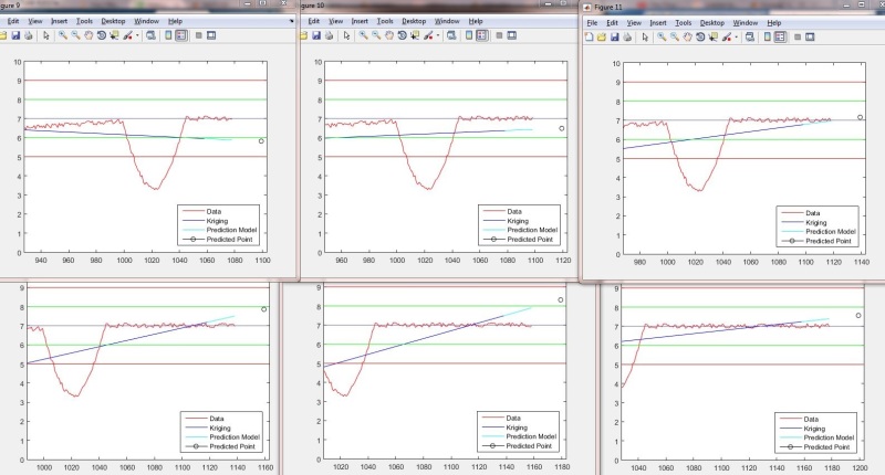
Right now, we've selected "kridging" for smoothing. I have some code that runs, though I'm not entirely sure it's doing what I really want. The data for testing code is fake, but one important anomaly is mimicked in the fake data: a sharp spike at about the 1000 sample mark lasting about 45 samples (see picture).
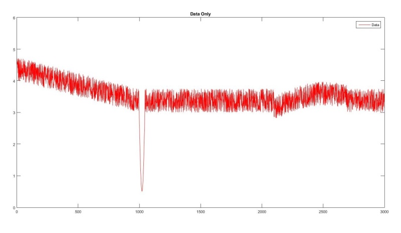
(y-data included as attachment...if anyone would like to plug it into code and run)
The question is...if you're running in data at real-time (almost) and want to ignore this or similar anomalies via computational and statistical methods, how should I go about doing this to maintain the trend from the first chunk of data, then continue on with smaller chunks of data being added. I have seen some other examples, but unfortunately nothing like this in MatLab that I can interpret. Here's the code I'm working with (thanks to developer of KrigingP.m):
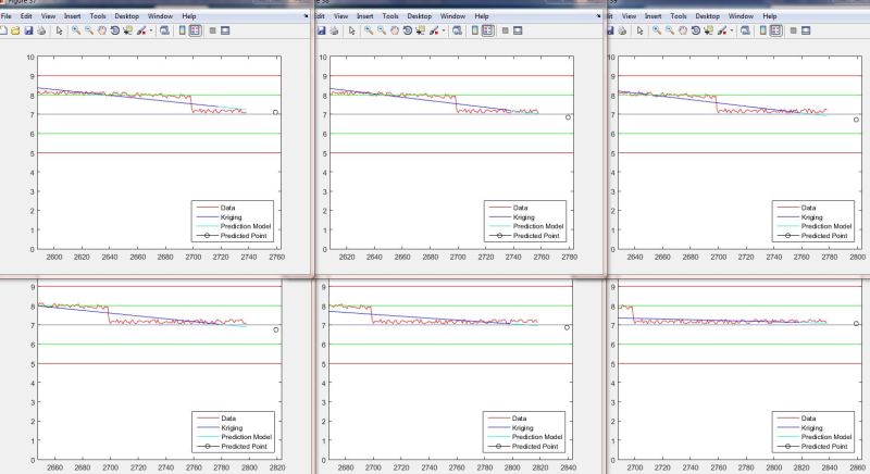
Here's an example output plot:
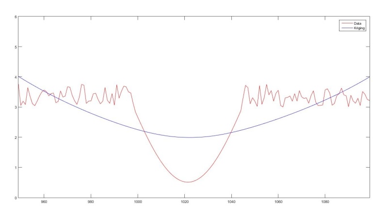
Later, this will be used to mathematically match a function to the trend and plug-in a prediction point some number of samples ahead (say maybe 20-50). Which is why it's important to travel across the anomaly with little influence to the trend.
More specifically, am I using the incorrect approach to handle the data under these conditions, and if so, could you please back it up with an explanation?
Thanks for any help you can provide (with statistical theory and/or coding).
So, no filters here, just creating a smoothed version (or trend) from the data (time is of the essence in this system's run-time). Starting theory in MatLab, then converting to C/C++ later (I speak MatLab, the other guys speak C; I wish I spoke both). I'll break it down; say you want to, for example:
1. Take in data for 150 (or N) samples, then after that you want to
2. generate a trend for initial data set (from initial sample to N)
3. Taking in new data for 20 (or F) of samples, consider past trend in
the new iteration of current trend (from F to N+F)...keep in mind,
is NOT like: moving F forward and taking a NEW trend across the new
data window, that would not take into account past trend.
4. Repeat 3.
Right now, we've selected "kridging" for smoothing. I have some code that runs, though I'm not entirely sure it's doing what I really want. The data for testing code is fake, but one important anomaly is mimicked in the fake data: a sharp spike at about the 1000 sample mark lasting about 45 samples (see picture).

(y-data included as attachment...if anyone would like to plug it into code and run)
The question is...if you're running in data at real-time (almost) and want to ignore this or similar anomalies via computational and statistical methods, how should I go about doing this to maintain the trend from the first chunk of data, then continue on with smaller chunks of data being added. I have seen some other examples, but unfortunately nothing like this in MatLab that I can interpret. Here's the code I'm working with (thanks to developer of KrigingP.m):
Code:
    x=0:1:1000; % sample number.
    %y= sorry, really long, included as txt link in post.
    sigma=2; % for use with Kriging function (Standard deviation).

    N=150; % total number of samples in each interpolation.
    F=20; % number of samples added/discarded each time.
    k=1; % separate counter, so I can move where loop starts and nothing breaks.
    m=0; % counter for conditional statement control.
    for j=950:1:length(y) % run through number of samples.
        if k==N+1 & m==0
            figure
            plot(x(j-N:j),y(j-N:j),'r-'); %plot data.
            hold on
            [Res]=KrigingP([x(j-N:j)' y(j-N:j)'],1,sigma,2,3); %calculate krig.
            yTrend(j-N:j)=Res(:,2);

            plot(x(j-N:j),yTrend(j-N:j),'b-'); % plot krig-ed interpolation.
            axis( [ x(j-N) x(j) 0 6 ] ); % for prediction: x(j+F+1)
            legend('Data','Kriging','Location','NorthEast');
            hold off
            m=m+1;
        elseif  (mod(k,F)==0) & (j < length(y)-N) & m==1 % do if j=every N and j<N from the end of y and (j>N, but not before first if has run)
            figure % ('units','normalized','outerposition',[0 0 1 1])
            plot(x(j-N:j),y(j-N:j),'r-'); %plot data.
            hold on
            [Res]=KrigingP([x(j-N:j)' y(j-N:j)'],1,sigma,2,3);
            yTrend(j-N:j)=Res(:,2);
            [Res]=KrigingP([x(j-N:j)' yTrend(j-N:j)'],1,sigma,2,3); %create trend
            yTrend(j-N:j)=Res(:,2);

            plot(x(j-N:j),yTrend(j-N:j),'b-'); % plot krig-ed interpolation.
            plot(Res(:,1),Res(:,2),'b-'); % plot krig-ed interpolation.
            axis( [ x(j-N) x(j) 0 6 ] );
            legend('Data','Kriging','Location','NorthEast');
            hold off
        elseif j>=1200 % early limit for code testing (less figures made).
            %fprintf('break'); % for debugging.
            break
        else
            %fprintf('else, j= %d \n',j); %for debugging
        end
        k=k+1;
    end
Here's an example output plot:

Later, this will be used to mathematically match a function to the trend and plug-in a prediction point some number of samples ahead (say maybe 20-50). Which is why it's important to travel across the anomaly with little influence to the trend.
More specifically, am I using the incorrect approach to handle the data under these conditions, and if so, could you please back it up with an explanation?
Thanks for any help you can provide (with statistical theory and/or coding).

![[wink] [wink] [wink]](/data/assets/smilies/wink.gif)