Postbuckling - meaning of LPF vs displacement plots 1

[FEA way]

Hi,

I would like to ask how the Load Proportionality Factor (LPF) vs displacement plots obtained from post-buckling analyses using Riks method should be interpreted. From what I've read actual load = applied load * LPF. So when I apply a critical buckling load obtained from eigenvalue (linear) buckling simulation to the imperfect geometry and get LPF vs displacement plot with LPF below 1 (about 0.8 - 0.9) all the time then does it mean that critical buckling load wasn't achieved (due to convergence issues) and thus the plot doesn't represent actual postbuckling behavior ? Or does it mean that the actual critical load value is smaller than what I've expected after linear buckling simulation and postbuckling was simulated ?

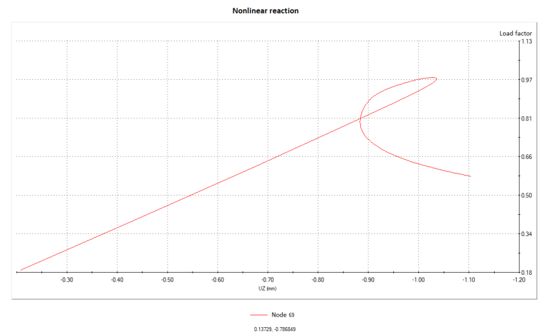
Here's an exemplary plot from such analysis (cylindrical shell under compression with trigger load of 1% of critical load applied in the direction of first buckling mode shape):

What does the loop at the end of it actually mean ?

Thanks in advance for your help

 

[SWComposites]

What analysis / code generated the plot?

It likely means the shell collapsed. Imperfect cylinders under compression will collapse at loads way below that predicted by eigenvalue analysis. See NASA SP-8007.

 

[ukbridge]

Im not really familiar with that type of structure but the graph doesn't look right to me.

A lot of the time these types of analysis require sitting down with the model and interrogating it but here are some tips:

1. It seems to me that the solution has failed to converge on a "correct" load path - this can sometimes happen with unstable systems when the global stiffness of the structure becomes very low. Looking at the animation will also help you identify if this might be happening.
2. Make sure you get enough load increments in near collapse - reduce it to say 0.01*load.
3. Make sure you define a maximum yield stress in your material properties i.e. so the software knows when the material undergoes plastic strain.
4. Also try defining an arbitrary low strain hardening gradient (say E/1000 even) - this can sometimes help convergence.
5. Make sure your software is using the arc-length procedure

From what I can see it looks like you're using LUSAS. (Disclaimer: I don't work for them!) Their customer support has always been excellent both from a customer-support and engineering perspective. I'd basically make ringing them your first port of call. There are also lots of useful guides on there to help you troublesheet nonlinear FE models.

 

[FEA way]

Thank you very much for replies. The analysis was done in SolidWorks Simulation and that's were I generated the plot too. Default properties of steel were used. No plastic data, only elastic constants but yield stress is always defined in the program (probably only for visualization as it shows the yield point value under the legend of von Mises stress plot).

What suggests that the analysis failed to converge ? That's the most important question for me - I need to know whether the postbuckling behavior was simulated correctly (as SWComposites suggested) or there was a convergence problem (as ukbridge states).

 

[ukbridge]

Hi FEA way,

Its hard for me to say without looking at the model. Its up to you to understand whether the graph "looks right" or not. To me, it does not - the transition from geometrically linear to nonlinear behaviour is very sudden and on a feel basis is not right to me.

The graph says to me "X Node (at the top of the shell?) undergoes linear vertical displacement with force. Then at a certain point undergoes some unloading which the response becomes somewhat stiffer. Its hard to picture it to be honest without more information.

Try doing the things I said above (adding plastic material data) - after all this is how steel actually behaves. Also:

1. Look at what nonlinear controls you are using (Total langrangian?)
2. Start with a simple column model and learn how to use that first.

At the end of the day this might be something thats outside your comfort zone (there is no shame in this btw - the other day I had to do seismic analysis and hadn't a clue until some bright chap sat down for half an hour with me to tell me the basics.)

Nonlinear analysis isn't something that should be used lightly - it requires a lot of experience and judgement to interpret. If you're struggling, sign off on the eigenvalue analysis until you get proper support/mentoring.

 

[ESPcomposites]

A few comments:

- The nonlinear analysis should have a result that is less than the Eigenvalue result. The goal is probably to determine just how much less.
- The perturbation (via geometry, load eccentricity, etc) is necessary for the nonlinear analysis. But it can't be arbitrary. The result will depend on the magnitude of the perturbation. You need a good way to quantify that and may want to do a sensitivity study to see how sensitive it is to the perturbation. That will give you an idea of accurate you need the perturbation magnitude to be.
- It is hard to say if the loop is correct. First off, you are only showing a single node and only the Z-component. You might want to try see how the out-of-plane components behave as well, especially at the location where the wall is collapsing. That plot may be more as you would normally expect.
- Rather than just looking at a single node (and a single displacement component), look at the tube's entire deformation as it goes through the loop. If it looks reasonable, then it is probably OK. After looking at that, and if you think it is correct, you may be able to find a better node(s) and corresponding displacement components (or RSS displacement) for a 2D plot.

Brian

http://www.structuralfea.com

 

[rb1957]

doesn't the plot show collapse at 97%, and whilst the model doesn't fall down the load capacity (load factor) is much reduced in the buckled state.

another day in paradise, or is paradise one day closer ?

 

[FEA way]

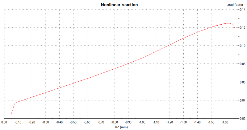
With plasticity included (values below) the plot is even stranger:

I don't like the idea of applying trigger load in the same analysis as buckling load (even though the trigger load is only 1% of the critical value) but it seems that there's no other way to introduce imperfections in SolidWorks Simulation. Apart from manually modifying the geometry of course.

Material data used in the simulation with von Mises plasticity:
- elastic modulus: 210 GPa
- tensile strength: 500 MPa
- yield strength: 200 MPa
- tangent modulus: 21 GPa
- hardening factor: 0

Other data I haven't mentioned yet:
- cylindrical shell size: 25 mm diameter, 80 mm height, 1 mm thickness
- fixed constraint at the bottom and compressive force (value from linear buckling: 424870 N) at the top
- trigger load - body force in the direction of first buckling mode (bending in negative direction of X axis): 4248 with amplitude (1 at the beginning of the simulation, decreasing to 0 at the end)
- direct sparse solver, arc length method (Newton-Raphson): max load pattern multiplier 100000000 (default), max displacement for translation DOF: 10 mm, max number of arc steps: 100, initial arc length multiplier 1

 

[ukbridge]

When you say "linear buckling" does that include allowances for geometric imperfections i.e. using the Perry-Robertston buckling curves? Or is "424870" simply your Pcr?

Physically the graph looks more "correct" to me. I'm not sure about your material properties:

1. 200MPa sounds quite low to me for yield strength but could well be the norm for these type of structures.
2. I've never personally specified a tangent modulus in any nonlinear analyses and cant comment.
3. Similarly I'm not sure what "hardening" factor exactly means either.
4. I've also never in the past relied on the full tensile strength in any nonlinear analyses.

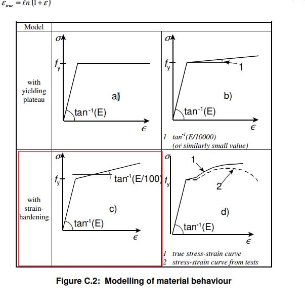
The graph indicates that plasticity is reached very early - check your numbers for your material parameters. In the past I've specified nonlinear material properties based on the below curves from the Eurocodes (EN 1993-1-5).

(Refer to the E/10000 figure not the one I've given in red). The UK National Annex only permits a maximum plastic strain of 5% (its up to you to work out whatever your code says).

In my program at least you simply enter your stress-strain curve (based on your data - check my numbers...) as:

Sigma,Epsilon
0,0
200, 200/210000
200+(0.05-200/210000)*210000/10000, 0.05.

If you post what the program is asking you to input I might be able to help more. Without stating the obvious check the manual, usually theres a worked example on these types of things.

gl

 

[ESPcomposites]

Some people call the Eigen solution "linear buckling", often as a way to distinguish it from "nonlinear buckling". However, "linear buckling" may not be the best way of describing the solution type (it is just an Eigen solution). While the load-deflection curve would be linear up the the point of buckling, you wouldn't have any use for the linear curve itself (at least not in this context). The Eigen solution calculates bifurcation buckling, which should be the upper end of the initial buckling load (note that there can be post-buckling phenomenon that can allow the actual structure to carry more load the Eigen solutions predicts, but that is after initial buckling occurs).

For nonlinear buckling, you do not use an Eigen solver. Instead, you can apply a load which you expect to exceed the structure's capability. You use a nonlinear solver as well. The first nonlinear aspect to consider is geometric nonlinearity. What happens is that the geometry will deform in such a manner as to increase out-of-plane deformations (i.e. an eccentricity of some sort). In order for this to occur, one must apply a perturbation (either via loading, geometry, etc.). This is the "imperfection" that is required (the eccentricity). If you don't do this, you may predict a load larger than the structure is capable of (real structures have imperfections). As the applied load is increased, so does the eccentricity (and the resulting moment caused by the eccentricity). This is a coupled effect and occurs in a beam-column (simple example to help one visualize it). As the eccentricity grows, it will become easier and easier to deform the part since the moment is rapidly increasing (it becomes unstable). Some structures can re-stabilize if there are other mechanisms at play (post-buckling). Once the out-of-plane deformations become large enough, the material will yield. So you can add that nonlinear consideration as well. But it is the geometric nonlinearity that is *drives* the material nonlinearity. However, adding the material nonlinearity will truncate the solution and prevent it from over-predicting the capability. If you were to perform a simple nonlinear beam analysis (with an eccentricity), you will see that once the beam starts moving out of the plane, the bending stresses quickly rise (it quickly goes from the onset of yielding to fully plastic with a small change in applied load). In the end, rather than having a sharp bifurcation buckling solution (Eigen solution), you would get a rounding of the curve as it becomes unstable (this is actual response of real structures with imperfections).

One of the best ways to determine if the nonlinear solution is correct is to observe the deformation of the structure as various load increments (and not just a single node and displacement component). Is the deformation reasonable? If so, you are on the right track. How does the deformation compare to the Eigen soution? If the predicted load (nonlinear solution) is not as expected, how sensitive is the solution to the magnitude of the perturbation? If it is sensitive, you will need to accurately define the perturbation. In my experience, that has been one of the biggest challenges with nonlinear buckling. While physically more representative, it may only be as good as your ability to accurately define the perturbation (depending on how sensitive it is).

Brian

http://www.structuralfea.com

 

[FEA way]

In SolidWorks Simulation, when I choose von Mises plasticity model, the table appears and the following data can be specified:
- elastic modulus
- Poisson's ratio
- tensile strength (I don't know if this one is actually used)
- yield strength
- tangent modulus
- thermal expansion coefficient (not important in this case obviously)
- mass density
- hardening factor

According to (rather poor) documentation the properties that need to be specified for bilinear stress-strain curve are:
- yield strength
- elastic modulus
- tangent modulus

For multilinear curve full stress-strain data should be defined of course. It is also stated that the hardening factor (called RK in documentation) is a ratio of kinematic and isotropic hardening. Thus for pure isotropic hardening it should be 0 (as in my case) while for pure kinematic hardening it should be 1.

From what I've read the tangent modulus is often defined as about 10% of elastic modulus.


When it comes to the size of imperfection, I agree that it's very important. From what I know it should be easier to achieve convergence with larger imperfection. It's hard to define it properly in SolidWorks since I can't use scaled mode shapes from eigenvalue buckling study but I decided to keep experimenting with the size of imperfection. It's all about experimentation after all.

 

[ukbridge]

I agree with ESPcomposites in terms of observing the global behaviour rather than a single node.

Also I agree the way in which you applied the perturbing mode might be a problem - a good software package should allow you to use the scaled deformed mesh of the eigenmode shape which should give you more "real" answers.

Nevertheless I think I understand now what "tangent" modulus means from

http://help.solidworks.com/2019/eng..._Plasticity_von_Mises_Model.htm?verRedirect=1

- its the strain hardening gradient as above in the extract I showed you (e.g. E/10000 for a negligible gradient, E/100 to actually consider the effects of strain hardening. Again to reiterate this is what is considered "good practice" in my own code (eurocodes) yours may vary.

To summarise:

1. I think you need to check your maths for your material parameters/units. It doesnt make sense to me that yield occurs at 4% of the load and plasticity occurs after an additional 6% or so give or take.

You need to replicate the curve I showed above in your software for the "bi-linear case". I would input in in terms of stresses and strains as I gave to you above (you can also do it in terms of E and sigma if you like - it does not matter as long as the math is right). If you do the maths the maximum plastic strain should be about 5%.

To start with use a tangent modulus of E/10000 (i.e. a negligible one) - start simple and build upwards.

2. Also make sure you apply the force that models the imperfection in a seperate loadcase, then use the deformed mesh from the end of that analysis as the starting point for your nonlinear analysis. There seems to be evidence of geometric nonlinearity from the graph you showed me though so I think (?) you're on the right lines for this one.

Keep at it gl

 

[ESPcomposites]

You can probably use a perfectly plastic model (no hardening) or a small tangent modulus. The amount of hardening probably won't make much of a difference because once it "gets moving" it usually goes quickly (that is why you can't stop a soda can from crushing mid way through the process). But I wouldn't get too caught up on trying to define the hardening accurately. But as a general note, if you did want to define it accurately, you would get that information from test data (such as MMPDS or other). You also want to be aware of is whether or not your codes requires the true stress/strain curve of the engineering stress/strain curve. Some codes are different and can even be different within the code itself (for example, Nastran uses one approach for SOL 106, but another for SOL 600).

The aspect you might care about the most is knowing that you have to truncate the solution when the material reaches its fracture strain. It is more likely to reach the fracture strain for a thicker wall than a thinner one. A thinner one may just elastically buckle and then exhibit plastic deformation but may not reach the fracture strain unless the solution is really pushed (but you are probably not concerned with that part of the solution). All that said, if the wall is thin enough, you will notice a decrease in load (probably the aspect you care about), before the material even yields...making the nonlinear material aspect moot. Again, you will have to interrogate the model, looking at the strains in the region that is collapsing and also observing the overall deformation. Good luck.

Brian

http://www.structuralfea.com

 

[rb1957]

the devil's in the details ...

I don't see why the 2nd graph is "even stranger" ... it points to collapse, doesn't it ?

yes, looking at the overall model deformations (particularly using dynamic display) is better for understanding behaviour ... but harder to show in a post (maybe attach a link to a video file ?).

another day in paradise, or is paradise one day closer ?