Excel formula help please 9

[Kenja824]

Cell A2 will have numbers with one or two letters mixed in. The letters are always together.

3L481
27H429
9SB75
etc...

In A1 I would like to place a formula that will return the numbers in the beginning along with the letters, but not the numbers after the letters.

3L
27H
9SB

I never know for sure what letters or numbers will be used.

I cant seem to find any examples of this.


Ken

http://www.OneGodLogic.com

My brain is like a sponge. A sopping wet sponge. When I use it, I seem to lose more than I soak in.

 

[SkipVought]

Here's an example that returns the numeric characters in a string up to the first non-numeric character...
[tt]
=LEFT(A2, MATCH(FALSE, ISNUMBER(VALUE(MID(A2, ROW(INDIRECT("1:" & LEN(A2))), 1))), 0) - 1)
[/tt]

Notice there's no SUBSTITUTE but there IS and ARRAY of the characters in A2, which is what the MID/ROW/INDIRECT functions returns to the formula.

The MATCH formula returns the offset up to the first alpha character as the character count for the LEFT function.

Skip,
[sub]
Just traded in my OLD subtlety...
for a NUance![/sub]

 

[3DDave]

Skip - Is it an array in A2 like ={"1","2","3","4...}? Where is the text that is being parsed? Is it also in A2?

 

[SkipVought]

A2 and following contain...

3L481
27H429
9SB75

Then [tt]MID(A2, ROW(INDIRECT("1:" & LEN(A2))), 1)[/tt] returns {"3", "L", "4", "8", "1"}

MATCH looks up FALSE from [tt]ISNUMBER(VALUE({"3", "L", "4", "8", "1"})), 0)[/tt] and returns the OFFSET of the first alpha character. Subtract 1 to giv you the number of numeric characters fir the LEFT function.

Skip,
[sub]
Just traded in my OLD subtlety...
for a NUance![/sub]

 

[3DDave]

Skip - I just found that formula you gave is required to be an array formula, so

{=LEFT(A2, MATCH(FALSE, ISNUMBER(VALUE(MID(A2, ROW(INDIRECT("1:" & LEN(A2))), 1))), 0) - 1)}

via Ctrl-Shift-Enter.

Still puzzling out what Microsoft Excel developers were thinking to get this sort of formula to work.

It's interesting the behind the scenes work that is going on; I'd like to say I've learned something applicable from this,
but I'm still missing the rules for when Excel is unwinding the arrays, such as this case of converting a single string into
a virtual column of individual characters.

 

[SkipVought]

What I find helpful in figuring out how a formula works is...

EDIT the formula.
SELECT an expression from within the formula like...
[tt]=LEFT(A2, MATCH(FALSE, ISNUMBER(VALUE(MID(A2, [highlight #FCE94F]ROW(INDIRECT("1:" & LEN(A2)))[/highlight], 1))), 0) - 1)[/tt]
Hit F9--this resolves the expression, displaying the value(s) produced by the expression.
Hit ESC--this returns the expression to your formula. IMPORTANT!!! DO NOT MISS THIS STEP OR YOU WILL LOOSE YOUR EXPRESSION!

Skip,
[sub]
Just traded in my OLD subtlety...
for a NUance![/sub]

 

[yakpol]

Skip, thanks for showing this technique. Implementing it I came up with this array formula. It looks weird, but works:
[tt]{=LEFT(A1,LEN(A1)-SUM(ISNUMBER(NUMBERVALUE(RIGHT(A1, ROW(INDIRECT("1:" & LEN(A1))))))*1))}[/tt]

 

[electricpete]

What I find helpful in figuring out how a formula works is...
[paraphrased: while editing, highlight subexpression and press F9 to see it evaluated, then escape when you're done]

LPS for that !!!
Who here hasn't spent a lot of time trying to figure out why a formula is working the way we expect.
I've done it waaay too many times, but never had the benefit of that tip.

=====================================
(2B)+(2B)' ?

 

[3DDave]

More Excel hocus-pocus.

It seems like it doesn't matter in the INDIRECT function if the argument is R1C1 format when the flag is specifically set to require A1
It also doesn't matter if it's a ROW or a COLUMN - I guess internally Excel just makes a list and ignores anything else, sometimes.
It doesn't matter if there are more entries than arguments (100 vs LEN(A2) = 5)
It doesn't matter if there is only one entry (change 100 to 1.)

The F9 trick isn't so reliable as to show what will happen.

Example:

=LEFT(A2, MATCH(FALSE, ISNUMBER(VALUE(MID(A2, [highlight #FCE94F]COLUMN(INDIRECT(100 & ":1",TRUE))[/highlight], 1))), 0) - 1)

reports that formulas cannot have more than 8192 characters. (Selecting the entire formula shows the
result "3", the left most set of numbers of "3L...")

But this:

=LEFT(A2, [highlight #FCE94F]MATCH(FALSE, ISNUMBER(VALUE(MID(A2, COLUMN(INDIRECT(100 & ":1",TRUE)), 1))), 0)[/highlight] - 1)

reports "2", the count to the first non-number.

Worse, this subsection works:
COLUMN(INDIRECT("1:1",TRUE))

This doesn't:
ROW(INDIRECT("1:1",TRUE))

and neither do
ROW(INDIRECT("1:1",FALSE)) or
COLUMN(INDIRECT("1:1",FALSE))

So if one explicitly requires R1C1 and uses R1C1, it fails.

 

[SkipVought]

It doesn't matter if there are more entries than arguments

I guess you're referring to the number of array elements as entries, but that has nothing to do with the
number of function arguments.

Yes, F9 can become useless if an array is too long. But in that case, one can carefully create test data
that tests the necessary conditions and limits.

The remainder, I'm not following. I don't give a flip about R1C1 notation.


Skip,
[sub]
Just traded in my OLD subtlety...
for a NUance![/sub]

 

[3DDave]

Skip - neither did the MS programmers. What I'm getting at is that if the software is used according to the MS documentation - IT FAILS.

Failing when used per the maker documentation is a huge problem.

No wonder Spoksky got it mostly right and then left.

 

[3DDave]

Skip, just to mention - "Yes, F9 can become useless if an array is too long. But in that case, one can carefully create test data
that tests the necessary conditions and limits."

F9 was failing on a sub-part of a formula that doesn't fail. It's not an array that is too long. It's creating a FORMULA that is too long in some
failure to evaluate the FORMULA. How you are going to test the FORMULA and avoid that is seemingly far more trouble than using VBA and making the
program explicit.

These are clever, brittle hacks.

The "entries" I created what I suspected was a 1 X 100 array for 5 elements. That is A-OK. Or maybe it thinks it is one cell at R100, C1. Can't tell
because it's all undocumented behaviors.

 

[IDS]

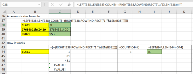
I have extracted the bits of this thread related to the original question in a blog post:

On long and short formulas and VBA

The screenshot below may be of interest:

Thanks to all for everything, even the side-discussions


Doug Jenkins
Interactive Design Services

http://newtonexcelbach.wordpress.com/

 

[SkipVought]

@Doug,

Again, you have rendered an invaluable concise solution that includes an inside-out, step by step
display that demonstrates your design of this excellent solution. Could be a tutorial.

It looks so easy and intuitive when broken down in steps. Of course it doesn't reveal the years
of knowledge and experience to know how to apply and arrange the capabilities of various functions.
Practice, practice, PRACTICE.

I think there's a limit in the length that a spreadsheet formula ought to be. It is a lot easier to design & write
VBA and a LOT easier to maintain and debug, IMNSHO. Humongous, hairy formulas are a bear to maintain and debug
let alone design. The documentation available in VBA code is valuable as well and ought to be supplied. I too often
fail in this area.

Skip,
[sub]
Just traded in my OLD subtlety...
for a NUance![/sub]

 

[SkipVought]

@3DDave,

I'm not that concerned about "undocumented behaviors."

The human kind is known for questioning and discovery. Whether a capability (a known feature) was designed in and then not documented,
is like amazing upon amazing! But like any tool, you must know and experience in use and experiment and push the envelope both of
your own capabilities and the capabilities of Excel.

I sure know that Excel has been used unwisely in the business world.

BTW, here's a link to a brief article regarding the start of MS Excel...

https://www.thedailybeast.com/micro...-software-that-changed-the-world-25-years-ago

I'd like to know more about how Excel was developed.

Skip,
[sub]
Just traded in my OLD subtlety...
for a NUance![/sub]

 

[3DDave]

Funny Skip,

I started with Lotus 1-2-3, then moved to Excel for Macintosh which was then re-written to run on Windows Runtime on MS-DOS. Still have
the floppy disks for the latter somewhere.

You should be concerned (but I know since you have a solution that works for you, you literally cannot be) about undocumented behaviors -
you are depending on them. They are unlikely to be designed in and just forgotten and more likely it is a flawed behavior side-effect,
like MCAS on the 737, that you are touting. Sometimes there's a reason some approach is poorly known.

Pushing the envelope makes for software that is not maintainable.

The human kind has been known to put metallic mercury, lead salts, methanol, and radium into food. Just because someone misuses something
isn't an excuse to find new ways to do so, no matter the claimed benefits of pushing an envelope.

 

[SkipVought]

@Doug,

Trimmed it down by two functions.
Removed ISNUMBER, substituted double unary for VALUE and substituted COUNT for SUM.
[tt]=LEFT(A7,LEN(A7)-COUNT(--(RIGHT(A7,ROW(INDIRECT("1:"&LEN(A7)))))))[/tt]

Your inside-out display approach helps visualize what's happening in the formula. Thanks!

Skip,
[sub]
Just traded in my OLD subtlety...
for a NUance![/sub]

 

[IDS]

Skip = sigh, I suppose I'll have to update my blog post now

The new even shorter formula in action:

Doug Jenkins
Interactive Design Services

http://newtonexcelbach.wordpress.com/

 

[3DDave]

Shorter:

=LEFT(A2,LEN(A2)-COUNT(--(RIGHT(A2,COLUMN(INDIRECT("1:1"))))))

As I wrote, the size of the target is meaningless, but it only is reduced using COLUMN().
ROW() fails to work correctly.

 

[SkipVought]

@3DDave,

Your "Shorter:" works.

However, the step-by-step as per Doug's solution, does NOT work to display the intermediate result.
Not sure what's happening. Undocumented? Undesigned?

Therefore, it is not as understandable as [tt]--(RIGHT(A2,ROW(INDIRECT("1:"&LEN(A23)))))[/tt]
Here you can actually SEE the array result. Much more useful. Much more desirable. Makes more sense.

Skip,
[sub]
Just traded in my OLD subtlety...
for a NUance![/sub]

 

[3DDave]

And here I thought you loved discovering new things.

None of this effort to avoid VBA with cryptic and undocumented side-effects makes more sense.